Specification for Kepler Orbit Propagation

1. Overview

1. Functions

The KeplerOrbit class calculates the satellite position and velocity with the simple two-body problem. We ignored any disturbances and generated forces by the satellite.
This orbit propagation mode provides the simplest and fastest orbit calculation for any orbit(LEO, GEO, Deep Space, and so on.).

2. Files

src/dynamics/orbit/orbit.hpp, cpp
- Definition of Orbit base class
src/dynamics/orbit/initialize_orbit.hpp, .cpp
- Make an instance of orbit class.
src/dynamics/orbit/kepler_orbit_propagation.hpp, .cpp
Libraries
- src/library/orbit/kepler_orbit.cpp, hpp
- src/library/orbit/orbital_elements.cpp, hpp

3. How to use

Select propagate_mode = KEPLER in the spacecraft's ini file.
Select initialize_mode as you want.
- DEFAULT : Use default initialize method (RK4 and ENCKE use position and velocity, KEPLER uses init_mode_kepler)
- POSITION_VELOCITY_I : Initialize with position and velocity in the inertial frame
- ORBITAL_ELEMENTS : Initialize with orbital elements

2. Explanation of Algorithm

1. `KeplerOrbit::CalcConstKeplerMotion` function

1. Overview

This function calculates the following constant values.
- Mean motion
- Frame conversion matrix from in-plane position to the inertial frame position

2. Inputs and outputs

Input
- Orbital Elements
- $\mu$ : The standard gravitational parameter of the central body
Output
- $n$ : Mean motion
- $R_{p2i}$ : Frame conversion matrix from in-plane position to the inertial frame position

3. Algorithm

Mean motion \[ n = \sqrt{\frac{\mu}{a^3}} \]
Frame conversion matrix from in-plane position to ECI position \[ R_{p2i} = R_z(-\Omega)R_x(-i)R_z(-\omega) \] \[ R_x(\theta) = \begin{pmatrix} 1 & 0 & 0 \\ 0 & \cos{\theta} & \sin{\theta} \\ 0 & -\sin{\theta} & \cos{\theta} \end{pmatrix} \] \[ R_z(\theta) = \begin{pmatrix} \cos{\theta} & \sin{\theta} & 0 \\ -\sin{\theta} & \cos{\theta} & 0 \\ 0 & 0 & 1 \end{pmatrix} \]

2. `KeplerOrbit::CalcOrbit` function

1. Overview

This function calculates the position and velocity of the spacecraft in the inertial frame at the designated time.

2. Inputs and outputs

Input
- $t$ : Time in Julian day
- Orbital Elements
- Constants
Output
- $\boldsymbol{r}_{i}$ : Position in the inertial frame
- $\boldsymbol{v}_{i}$ : Velocity in the inertial frame

3. Algorithm

Calculate mean anomaly $l$[rad] \[ l = n * (t-t_{epoch}) \]
Calculate eccentric anomaly $u$[rad] by solving the Kepler Equation
- Details are described in KeplerOrbit::SolveKeplerFirstOrder
Calculate two dimensional position $x^{*}$, $y^{*}$ and velocity $\dot{x}^{*}$, $\dot{y}^{*}$ in the orbital plane \[ \begin{align} x^* &= a(\cos{u}-e)\\ y^* &= a\sqrt{1-e^2}\sin{u}\\ \dot{x}^* &= -an\frac{\sin{u}}{1^e\cos{u}}\\ \dot{y}^* &= an\sqrt{1-e^2}\frac{\cos{u}}{1^e\cos{u}}\\ \end{align} \]
Convert to the inertial frame \[ \begin{align} \boldsymbol{r}_{i} &= R_{p2i}\begin{bmatrix} x^* \\ y^* \\ 0 \end{bmatrix}\\ \boldsymbol{v}_{i} &= R_{p2i}\begin{bmatrix} \dot{x}^* \\ \dot{y}^* \\ 0 \end{bmatrix}\\ \end{align} \]

3. `KeplerOrbit::SolveKeplerFirstOrder` function

1. Overview

This function solves the Kepler Equation with the first-order iterative method.
Note: This method is not suited to the high eccentricity orbit. It is better to use the Newton-Raphson method for such a case.
- From v6.0.0 we have SolveKeplerNewtonMethod and use it. The detail of the method will be write.

2. Inputs and outputs

Input
- $e$ : eccentricity
- $l$ : mean anomaly [rad]
- $\epsilon$ : threshold for convergence [rad]
- Limit of iteration
Output
- $u$ : eccentric anomaly [rad]

3. Algorithm

Set the initial value of eccentric anomaly as follows
- $u_0=l$
Calculate $u_{n+1}$ with the following equation \[ u_{n+1} = l + e\sin{u_n} \]
Iterate the calculation until the following conditions are satisfied
- $|u_{n+1} - u_{n}| < \epsilon$
- The iteration number over the limit of iteration

4. `OrbitalElements::CalcOeFromPosVel` function

1. Overview

This function calculates the orbital elements from the initial position and velocity in the inertial frame.

2. Inputs and outputs

Input
- $\mu$ : The standard gravitational parameter of the central body
- $t$ : Time in Julian day
- $\boldsymbol{r}_{i}$ : Initial position in the inertial frame
- $\boldsymbol{v}_{i}$ : Initial velocity in the inertial frame
Output
- orbital element

3. Algorithm

$\boldsymbol{h}_{i}$ : Angular momentum vector of the orbit \[ \boldsymbol{h}_{i} = \boldsymbol{r}_{i} \times \boldsymbol{v}_{i} \]
$a$ : Semi-major axis \[ a = \frac{\mu}{2\frac{\mu}{r} - v^2} \]
$i$ : Inclination \[ i = \cos^{-1}{h_z} \]
$\Omega$ : Right Ascension of the Ascending Node (RAAN)
- Note: This equation is not support $i = 0$ case. \[ \Omega = \sin^{-1}\left(\frac{h_x}{\sqrt{h_x^2 + h_y^2}}\right) \]
$x_{p}, y_{p}$ : Position in the orbital plane \[ \begin{align} x_{p} &= r_{ix} \cos{\Omega} + r_{iy} \sin{\Omega};\\ y_{p} &= (-r_{ix} \sin{\Omega} + r_{iy} \cos{\Omega})\cos{i} + r_{iz}\sin{i} \end{align} \]
$\dot{x}_{p}, \dot{y}_{p}$ : Velocity in the orbital plane \[ \begin{align} \dot{x}_{p} &= v_{ix} \cos{\Omega} + v_{iy} \sin{\Omega};\\ \dot{y}_{p} &= (-v_{ix} \sin{\Omega} + v_{iy} \cos{\Omega})\cos{i} + v_{iz}\sin{i} \end{align} \]
$e$ : Eccentricity \[ \begin{align} c_1 &= \frac{h}{\mu}\dot{y}_p - \frac{x_p}{r}\\ c_2 &= -\frac{h}{\mu}\dot{x}_p - \frac{y_p}{r}\\ e &= \sqrt{c_1^2 + c_2^2} \end{align} \]
$\omega$ : Argument of Perigee \[ \omega = \tan^{-1}\left(\frac{c_2}{c_1}\right) \]
$t_{epoch}$ : Epoch [Julian day] \[ \begin{align} f &= \tan^{-1}\left(\frac{y_p}{x_p}\right) - \omega\\ u &= \tan^{-1}\frac{\frac{r \sin{f}}{\sqrt{1-e^2}}}{r\cos{f} + ae}\\ \end{align} \] \[ \begin{align} n &= \sqrt{\frac{\mu}{a^3}}\\ dt &= \frac{u - e\sin{u}}{n}\\ t_{epoch} &= t - \frac{dt}{246060} \end{align} \]

3. Results of verifications

1. Comparison with RK4

1. Overview

We compared the calculated orbit result between RK4 mode and Kepler mode. In the RK4 mode, all disturbances are disabled since the Kepler mode ignores them.
In the Kepler mode, we verified the correctness of both initialize modes (ORBITAL_ELEMENTS and POSITION_VELOCITY_I).

2. Conditions for the verification

sample_simulation_base.ini
- The following values are modified from the default.
```
EndTimeSec = 10000
LogOutPutIntervalSec = 5
```
SampleDisturbance.ini
- All disturbances are disabled.

SampleSat.ini

The following values are modified from the default.

propagate_mode is changed for each mode.

Orbital elements for Kepler

semi_major_axis_m = 6794500.0
eccentricity = 0.0015
inclination_rad = 0.9012
raan_rad = 0.1411
arg_perigee_rad = 1.7952
epoch_jday = 2.458940966402607e6

Initial position and velocity (compatible value with the orbital elements)

init_position(0) = 1791860.131
init_position(1) = 4240666.743
init_position(2) = 4985526.129
init_velocity(0) = -7349.913889
init_velocity(1) = 631.6563971
init_velocity(2) = 2095.780148

3. Results

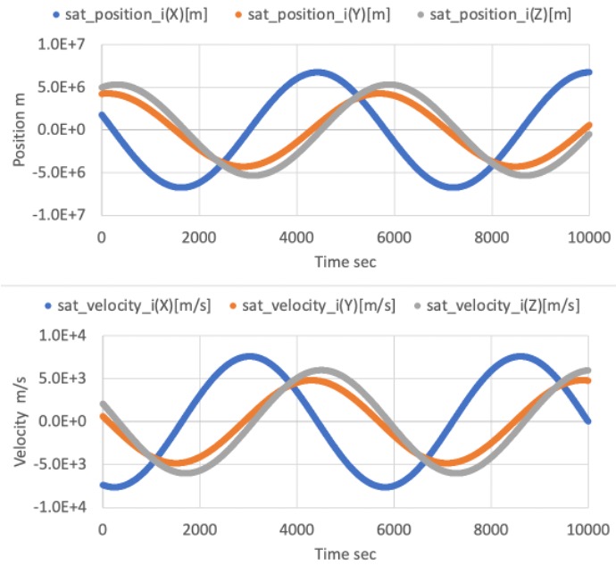
The following figure shows the orbit calculation result of Kepler mode with ORBITAL_ELEMENTS initialize mode.
- The result looks correct.
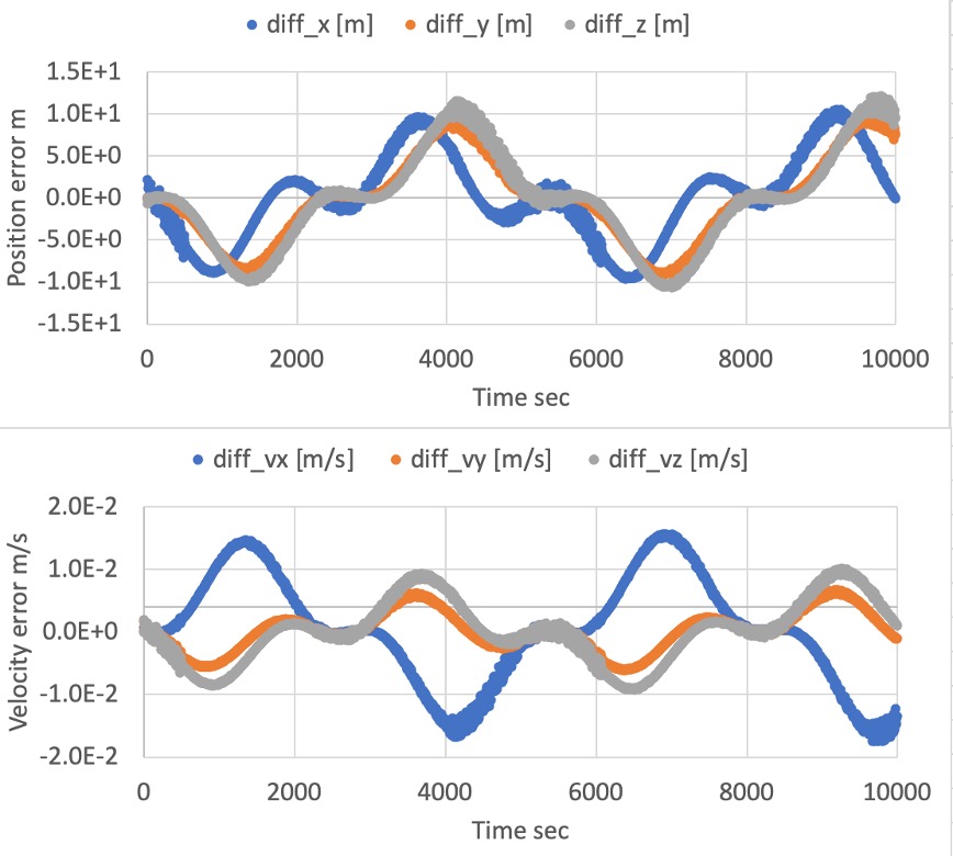
The difference between Kepler mode with ORBITAL_ELEMENTS initialize mode and RK4 mode is shown in the following figure.
- The error between them is small (less than 10m), and we confirmed that the calculation of Kepler orbit is correct.
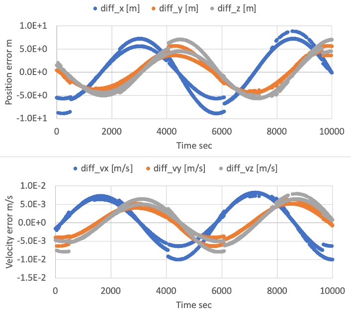
The following figure shows the difference between Kepler orbit calculation with ORBITAL_ELEMENTS and POSITION_VELOCITY_I initialize mode.
- The error between them is small (less than 10m), and we confirmed that the initializing method is correct.

4. References

Hiroshi Kinoshita, "Celestial mechanisms and orbital dynamics", ch.2, 1998 (written in Japanese)

S2E documents