Overview
Coding Convention of S2E
Formatter
- We use ClangFormat for S2E.
- We selected
Googlebase style with small modifications. - Details are written in .clang-format.
- We selected
Naming Rules
-
Now discussing
- The following rules are follows until the new naming rule is decided.
- Several old files do not follow the rules.
- We are discussing follow the Google C++ Style Guide with small modifications.
-
File and directory Name
snake_case- C++ files should end in
.cpp, and header files should end in.hpp.
-
Macro (define)
- Snake case with capital case
SNAKE_CASE
-
Name of the class
CamelCase
-
Variable name
- Snake case with lower case
snake_case
-
Constant name (not a define but a constant)
- Add k at the beginning and the rest is CamelCase
kCamelCase
-
Member variables in the class
- Snake case with lower case end with
_ snake_case_
- Snake case with lower case end with
-
Methods (functions) in the class
CamelCase
-
The #define Guard
- Apply Google C++ Style Guide.
#pragma onceis prohibited
Documentation
- Use Doxygen
- Use Markdown for Doxygen
- Examples:
- https://developer.lsst.io/cpp/api-docs.html
Initialization files (.ini files)
- Comments
- Use //
Abbreviations
- Basically, we follows the Naming Rules in the Google Style Guide
- Single character abbreviations are prohibited.
- Examples:
q = quaternion,v = velocityare prohibited.
- Examples:
- We do not recommend to use abbreviations for one word cutting the word.
- Examples:
pos = position,quat = quaternionare not recommended. - The following abbreviations are available as exceptions since they are widely used in the math, science, and technology field.
max: maximummin: minimuminit: initial, initializecalc: calculate, calculation
- Examples:
- Abbreviation only file name is not recommended.
- Examples
ode.hppshould be written asordinary_differential_equation.hppgnssr.hppis not recommended, butgnss_receiver.hppis available since we can guess the abbreviation meaning from the context.
- Examples
- Write the full words in the comment when you use abbreviations.
- Available abbreviations are decided during review processes.
- Examples of available abbreviations with comments
EKF: Extended Kalman FilterGNSS: Global Navigation Satellite System
- Examples of available abbreviations with comments
- Abbreviations to show the frame and the unit are available.
- Examples of frame
i: Inertial frameb: Body fixed framec: Component fixed frameecef: Earth Centered Earth Fixed framelvlh: Local Vertical Local Horizontalrtn: Radial-Transverse-Normal
- Examples of unit:
Nm,rad/s,m/s2,degC
- Examples of frame
- Available abbreviations
S2E: Spacecraft Simulation EnvironmentAOCS: Attitude and Orbit Control SystemCDH: Command and Data Handling
Format to write specification documents
0. General rule
- The file name should be
Spec_CamelCase.mdin the Specifications directory. - Please use the markdown format.
- Because GitHub started to support math description (link), we need to describe equations suit with the rule of GitHub and MathJax.
1. Overview
1. Features
- Write an overview of features to be realized using the class or library here clearly.
2. Related files
- Enumerate all related codes and input files here
3. How to use
- Write how to use the class or functions
2. Explanation of Algorithm
Write important algorithms for the class, the library, or each function. Please use equations, figures, reference papers for easy understanding.
1. Name of class, structure, and function
1. Overview
- Please summarize the
2. Inputs and Outputs
- Please list up inputs and outputs
3. Algorithm
- Please use math description when you need as follows $$\dot{\boldsymbol{x}}=f(\boldsymbol{x},t)$$
\[ \dot{\boldsymbol{x}}=f(\boldsymbol{x},t) \]
- you can also use inline equation as $x=y$
4. Note
2. Name of function
1. Overview
2. Inputs and Outputs
3. Algorithm
4. Note
3. Name of function
1. Overview
3. Results of verifications
1. Name of verification case
1. Overview
- please write a reason why the author does the verification
2. conditions for the verification
- input files
- initial values
3. result
- please use figures to show the results clearly
- Upload the figure files in
figsdirectory- Note: the figure size should be smaller than several hundred K Bytes
- Smaller is better
- Link the figure file with relative path
- Note: the figure size should be smaller than several hundred K Bytes
4. References
How to build and execute with Visual Studio
1. Overview
This document explains how to build and execute the Visual Studio environment with CMake. Currently, we recommend using VS2022, but users can use VS2019 and VS2017 with minor modifications.
- Related files
- ./CmakeLists.txt
- Base file for CMake
- ./CMakeSettings.json
- Setting file for VS to use CMake
- Other CMakeLists.txt in subdirectories
- ./CmakeLists.txt
2. Environment Construction of Visual Studio
- Install Visual Studio 2022
- Select the following
Workloadswhen installing the VS2022Desktop development with C++
- Select the following
- Clone s2e-core
- Please use
the latest release version. - The following procedure possible does not work for
The latest develop branch.
- Please use
- Check that the
ExtLibrariesdirectory is in the same directory as thes2e-corelike below.├─ExtLibraries └─s2e-core
- If not, please follow the procedure below to make
ExtLibraries- Launch VS 2022
- Open the CMake file for the
ExtLibraries- Click
Files/Open/CMake. - Select the following
s2e-core/ExtLibraries/CMakeLists.txt.└─s2e-core └─ExtLibraries └─CMakeLists.txt - Wait a moment until the
CMake generationis finished.
- Click
- Install the
ExtLibraries- Select
CMakeLists.txtby right-clicking in the VS'sSolution Explorer. - Click the
Installcommand. - Wait a moment until the installation is successfully finished.
- Select
- Check that the
ExtLibrariesdirectory is in the same directory as thes2e-core - Check there are
cspiceandnrlmsise00directories in theExtLibrarieslike below.├─ExtLibraries │ └─cspice │ └─GeoPotential | └─nrlmsise00 └─s2e-core
- If not, please follow the procedure below to make
3. The flow of building and execution in Visual Studio 2022
-
Launch VS 2022
-
Open the S2E project
- Click
File/Open/CMake. - Select
s2e-core/CMakeLists.txtat the top directory of the cloned S2E. - Wait a moment until the
CMake generationis finished.
- Click
-
Build the S2E
- Select
CMakeLists.txtby right-clicking in the VS'sSolution Explorer. - Click the
Buildcommand. - Wait a moment until the build is successfully finished.
- Select
-
Check errors
- When users edit the codes, please check the error and fix them.
-
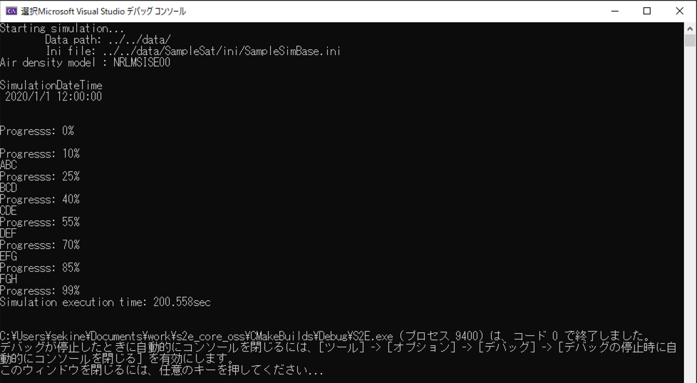
Run the program
- Select
S2E.exeas the red circle of the following figure.
- Click the
green play buttonin the red circle to run the S2E. - A console window is opened, and users can see the S2E's running status.
- Select
-
Check log files
- Open the
./data/***/logs/logs_***directory. - Open the CSV file to check the log output of the S2E.
- Open the
4. Note
- For VS2019 users
- Please edit the compiler setting in
CMakeSetting.jsonas"generator": "Visual Studio 16 2019".
- Please edit the compiler setting in
- For VS2017 users
- Please edit the compiler setting in
CMakeSetting.jsonas"generator": "Visual Studio 15 2017". - Users also need to edit the
cmake_minimum_requiredversion from 3.13 to 3.10 in all CMakeList, including the files in subdirectories. The VS 2017 does not support version 3.13, and you may see manywarningswhen you use CMake Version 3.10.
- Please edit the compiler setting in
How to compile with Ubuntu in Docker
1. Overview
- Docker is useful for the easy setup of the compile environment for S2E.
- Both Windows and Mac users can use the same environment and get the same result by using the docker container.
- We selected Ubuntu as an OS in the docker image and GCC/G++ as a compiler for S2E.
Note: We currently use a 32bit compiler for S2E since flight S/Ws are usually executed on a 32bit microcomputers. - We recommend using Visual Studio Code as an editor for the environment.
- This document explains a setup sequence of the docker environment for S2E.
- Note: For a detailed explanation of Docker and VSCode's Extensions, please see the latest and official information.
2. Install Required Application
2.1. Docker
- Go to the install web page of Docker.
- Install
Docker for WindowsorDocker for Macto suit your platform.
2.2. Visual Studio Code (VS Code)
- Go install web page of VS Code.
- Install
Visual Studio Codeto suit your platform. - Install following extensions
- Remote-SSH
- CMake
- CMake Tools
- C/C++
- Following extensions are also useful
- Code Spell Checker
2.3. For Mac users
- Install the
coreutilsto use therealpathcommand insetup_docker.sh- Use the
brew install coreutilscommand when you haveHomebrew
- Use the
3. A Sequence of environment setting
3.1. Working directory setting
- Create a
workdirectory as a working directory. - Clone s2e-core in the
workdirectory. - Add the
workdirectory in thefile sharingdirectory of Docker.- Note: This setting does not exist in the latest Docker and WSL2 environments in Windows, so it is not necessary.
3.2. Make Docker image and container
- Launch
git bash(for windows users) orterminal(for Mac users) - Move
/s2e-core/scripts/Docker_Ubuntudirectory - Edit
Dockerfileorsetup_docker.shwhen you want to change the directory name, the user name of the container, and other settings. - Execute
./setup_docker.sh buildto make images - Check created images (
issl(andubuntu))- command:
docker images
- command:
- Execute
./setup_docker.sh run_coreto make the container - Check created container (
issl:latest)- command:
docker ps -a
- command:
- Check the dashboard of Docker as follows.

3.3. SSH connects with VS Code
- Launch
VS Codeand open a new window. - Click the
Remote Explorericon on the left side.- Note: the icon looks like a monitor
- Click the
gearicon ofSSH TARGETSand select the config file you want to edit- Default:
C:\Users\UserName\ssh\configorUser/UserName/ssh/config
- Default:
- Edit the config file as follows
Host issl-1 HostName localhost User s2e Port 2222 - Save the config file and check a new SSH target
issl-1is made in the explorer - Click
Connect to Host in New Windowicon on right side ofissl-1 - Enter the password
s2ewhen required - See left bottom icon
SSH:issl-1to confirm the connection - Open the
workdirectory in the container by usingOpen folder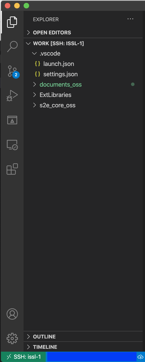
3.4. Download External Libraries
Note : This sequence was integrated within the docker build process, so this is currently unnecessary.
- S2E has several script files to get external libraries.
- For this ubuntu/docker platform, users should use script files in
scripts/Commondirectory andscripts/Docker_Ubuntudirectory. - Users can execute most of the script files with
git bashorterminalin the outside of the container, but users should executescripts/Common/download_nrlmsise00_src_and_table.shinside the container to use the same compiler. - Click
Terminal > New terminalin the menu bar of VS Code. - Select
bashterminal at the bottom window. - Execute
./s2e-core/scripts/Common/download_nrlmsise00_src_and_table.sh. - See
ExtLibrariesto confirm the NRLMSISE library is generated.
3.5. Build S2E
- Install the following extensions in the
issl-1 SSH connection
Even if the extensions were already installed in local VS code, you also need to install them in theSSH connection.- C/C++
- CMake
- CMake Tools
Note : You need to reload VS Code after installing new extensions
- Edit setting of
CMake Toolsinissl-1Cmake Build Directory: ${workspaceFolder}/s2e-core/build/Debug - After
CMakeandCMake Toolsare installed, VS Code requires you to configure the building environment withCMakeList.txt. Please selectyes. However, there is noCMakeList.txtfile in theworkdirectory, and VS Code requires you to locateCMakeList.txt, so please select theCMakeList.txtfile ins2e-coredirectory.- This setting is written in
.vscode/settings.json - You can directly edit the
settings.jsonas follows{ "cmake.sourceDirectory": "${workspaceFolder}/s2e-core", "cmake.buildDirectory": "${workspaceFolder}/s2e-core/build/Debug" }
- This setting is written in
- Select
GCC 11.2.0as a kit (compiler)- Note: Users can also choose other GCC versions.
- Select
CMake [Debug]and check the configuration is successfully done. - Build S2E
- If you want to clean up, please use
CMake: Cleancommand.
- If you want to clean up, please use
- Move to
build/Debugdirectory withTerminalin VS Code. - Execute
./S2Eor click therunicon at the bottom. - Check the
data/logdirectory to confirm log file output.
4. Debug with VS Code
- Select
Run > Start Debuggingin the menu bar. - Select
C++(GDB/LLDB)debugger- If
C++(GDB/LLDB)is not shown, please open a CPP file and selectRun > Start Debuggingagain. .vscode/launch.jsonwill be created.
- If
- Edit as follows.
"program": "${workspaceFolder}/s2e-core/build/Debug/S2E", "cwd": "${workspaceFolder}/s2e-core/build/Debug", - Select
Run > Start Debuggingagain. - Check the
data/logdirectory to confirm log file output. - You can use breakpoints in the VS Code editor.
How to compile with OSX Environment
How to download and make NRLMSISE00 Library
1. Overview
- NRLMSISE00 is an atmosphere model to calculate an air density, considering the solar activity.
- C language version of NRLMSISE00 is a mandatory library for S2E to calculate the atmosphere density around the Earth.
- How to use NRLMSISE00 is written in the Specification of Atmosphere model.
- Note From the s2e-core v5.0.0 we provide the CMake file to download and install the external libraries and recommend to use it since it is simpler. So users do not need to execute the following process.
2. How to set up NRLMSISE00 for S2E [OLD Descriptions]
-
In any environment, run
s2e-core/scripts/Common/download_nrlmsise00_src_and_table.sh- Source codes of NRLMSISE00 and
SpaceWeather.txtwill be downloaded, andlibnrlmsise00.awill be made for Linux and OSX.- Users have to compile the codes using the same compiler with S2E. After these codes are downloaded, you can directly compile them by using makefile in the
ExtLibraries\nrlmsise00\src.
- Users have to compile the codes using the same compiler with S2E. After these codes are downloaded, you can directly compile them by using makefile in the
- If you use Windows, a bash terminal for Windows (e.g. Git bash, WSL, MSYS) is needed to run this script, and you need to run an additional script. Proceed to Step 2.
- Source codes of NRLMSISE00 and
-
For Windows Visual Studio users, run
s2e-core/scripts/VisualStudio/make_nrlmsise00_VS32bit.batafter the process 1.- VS command prompt will be launched, then run
scripts/VisualStudio/make_libnrlmsise.batin VS command prompt. libnrlmsise.lib, which is the library for Windows Visual Studio will be made.- At the end of the procedure, you may see "指定されたバッチ ラベルが見つかりません - END". If there is
libnrlmsise00.libin the right place and all the files are in the right place, you may ignore this message.
- VS command prompt will be launched, then run
-
Check your directories are as follows.
  ├─ExtLibraries
  │  └─nrlmsise00
  │      ├─table
  |      |  └─SpaceWeather.txt
  │      ├─lib
  |      |  |─libnrlmsise00.a
  |      |  └─libnrlmsise00.lib
  │      └─src
  |         └─nrlmsise-00.h
  └─s2e-core
How to download CSPICE Library
1. Overview
- SPICE is a system to combine the most accurate space geometry and event data with space mission analysis, observation planning, or science data processing software developed by NASA.
- CSPICE is the C language version of SPICE and mandatory library for S2E to get planet information.
- Note From the s2e-core v5.0.0, we provide the CMake file to download and install the external libraries and recommend to use it since it is simpler. So users do not need to execute the following process.
2. How to set up CSPICE Library for S2E [OLD Descriptions]
Note: Users can use the script file to automatically set up the following process in the s2e-core/script directory. If the script does not work, please see the following process.
- Make directories as follow
  ├─ExtLibraries
  │  └─cspice
  │      ├─cspice_xxx
  │      │  └─lib
  │      ├─generic_kernels
  │      └─include
  └─s2e-core
-
xxx is depends on your compile environment
xxx = msvsfor Microsoft Visual Studioxxx = cygwinfor Cygwin gCCxxx = unixfor Linux gCC
-
Download library and compile
- Download
cspice.zipfrom NAIF Toolkit, and unzip. - You need to choose a link suit with your compile environment
- Copy
includedirectory intocspicedirectory - Copy
liborlib64directory intocspice_***directory- VS 2019 users need to compile the library before copying the
lib- launch following command prompt for VS2019 compile from the start menu of Windows
- 32bit:
x86 Native tools command prompt for VS2019 - 64bit:
x64 Native tools command prompt for VS2019
- 32bit:
- Move to the unzipped directory and execute
makeall.bat
- launch following command prompt for VS2019 compile from the start menu of Windows
- VS 2019 users need to compile the library before copying the
- Download
-
Download kernel files
- Download the following kernel files from NAIF Generic Kernels, and copy them to the directories
- Each kernel file can be updated for the latest one, but we have not confirmed it yet.
├─generic_kernels │ ├─lsk │ └─naif0010.tls │ ├─pck │ └─de-403-masses.tpc │ └─gm_de431.tpc │ └─pck00010.tpc │ └─spk │ └─planets │ │ └─de430.bsp - Download the following kernel files from NAIF Generic Kernels, and copy them to the directories
Note: When you change the directory or file name, you should modify s2e-core/CMakeLists and PlanetSelect.ini
Getting Started
1. Overview
- This tutorial explains how to use the S2E simulator without any source code modification.
- Users can start this tutorial just after users clone the s2e-core repository.
- The supported version of this document
- Please confirm that the version of the documents and s2e-core is compatible.
2. Clone, Build, and Execute
- Clone s2e-core.
- Read
README.mdto check the overview of S2E. - Build and execute the
s2e-coreby referring following documents depends on your development environment.
3. Check log output
- Check
./data/sample/logsto find CSV log output file- The file name includes executed time as
YYMMDD_HHMMSS_default.csv - The included executed time is defined by the user computer settings.
- The file name includes executed time as
- Open the CSV log file
- You can see the simulation output
- The meaning of each value is described in the first row
- A general rule of the header descriptions are summarized here.
- You can write a graph from the CSV file as you need.
- You can find plot examples written in Python in the
scripts/Plotdirectory. - Please see How to Visualize Simulation Results for more details.
- You can find plot examples written in Python in the
4. Edit Simulation Conditions
- Move to
./data/sample/initialize_filesdirectory - You can find the several initialize files (INI files). In these initialize files, simulation conditions are defined, and you can change the conditions without rebuild of S2E by editing the initialize files.
- Open
sample_simulation_base.ini, which is the base file of the initialize files.- In this base file, other initialize files are defined.
- You can see simulation conditions as time definitions, randomize seed definitions, etc.
- Open
sample_satellite.ini, which is the file to set the spacecraft parameters. - Edit the value of angular momentum
initial_angular_velocity_b_rad_s(0-2)in the[Attitude]section as you want. - Set the value of
initialize_modetoMANUALif it isCONTROLLED. - Rerun the
s2e-corewithout a rebuild - Check the new log file in
./data/sample/logsto confirm the initial angular velocity is changed as you want. - Of course, you can change other values similarly.
5. Edit Simulation Conditions: Disturbances
- Move to
./data/sample/inidirectory again - Open
sample_disturbance.ini, which defines conditions to calculate orbital disturbance torques and forces- Currently, S2E supports the following disturbances:
- Gravity Gradient torque
- Magnetic Disturbance torque
- Air drag torque and force
- Solar radiation pressure torque and force
- Geo Potential acceleration
- Third body gravity acceleration
- Currently, S2E supports the following disturbances:
- You can select
ENABLEorDISABLEof calculation and log output for each disturbance - Edit all
calculationparameters of each disturbance ascalculation = DISABLE - Rerun the
s2e-corewithout a rebuild - Check the new log file in
./data/sample/logsto confirm the spacecraft is not affected by any disturbance torque and the angular velocity and quaternion are not changed. You can also plot by following command and see all the disturbance torque and force are zero. (assuming you already created apipenvvirtual environment)# Windows cd scripts/Plot pipenv run python .\plot_disturbance_torque.py --file-tag <log file tag> pipenv run python .\plot_disturbance_force.py --file-tag <log file tag> - Edit
calculationof [THIRD_BODY_GRAVITY] ascalculation = ENABLE - Rerun the S2E_CORE without a rebuild
- Rerun the python script to check the third body gravity is generated.
6. Edit Simulation Conditions: Orbit
-
Move to
./data/sample/inidirectory -
Open
sample_satellite.iniand see the[Orbit]section, which defines conditions to calculate orbit motion- Currently, S2E supports several types of orbit propagation. Please see Orbit specification documents for more details.
-
Please set the parameters as follow:
propagate_mode = SGP4: SGP4 Propagatorinitialize_modeis not used in the SGP4 propagate mode.- TLE: ISS orbit (default)
-
To get a long-term orbit simulation data, edit the following simulation time settings in
sample_simulation_base.inisimulation_duration_s = 6000log_output_period_s = 10(to decrease the output file size)
-
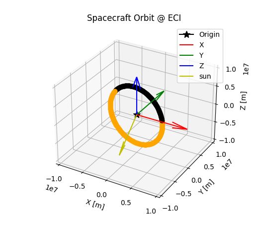
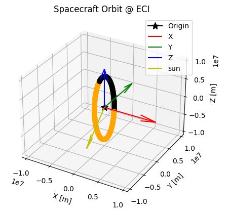
To visualize the orbit result, execute the
plot_satellite_orbit_on_miller.pyandplot_orbit_eci.pyby following command. You can see the plots as follows. Please see general documents for more details on visualization of simulation results.# Windows cd scripts/Plot pipenv run python .\plot_satellite_orbit_on_miller.py --file-tag <log file tag> pipenv run python .\plot_orbit_eci.py --file-tag <log file tag>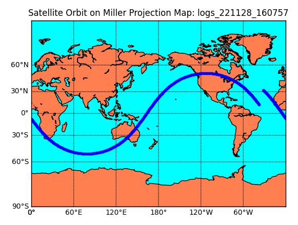
-
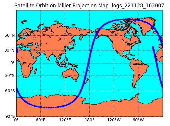
Change TLE as you want
- Example: PRISM (Hitomi)
tle1=1 33493U 09002B   22331.71920614  .00003745  00000-0  29350-3 0  9995
tle2=2 33493  98.2516 327.9413 0016885   9.3461 350.8072 15.01563916753462
- Example: PRISM (Hitomi)
-
Rerun the
s2e-corewithout a rebuild -
Check the new log file in
./data/sample/logsto confirm the spacecraft position in ECI framespacecraft_position_iis changed. -
To visualize the orbit result, execute the
plot_satellite_orbit_on_miller.pyandplot_orbit_eci.py. You can see the different plots as follows.
7. Edit Simulation Conditions: Environment
- Move to
./data/sample/inidirectory - Open
sample_local_environment.ini, which defines conditions to calculate the environment around the spacecraft- Currently, S2E supports the following environment models:
- Celestial information: CSPICE
- Geomagnetic field model: IGRF with random variation
- Solar power model: Considering solar distance and eclipse
- Air density: NRLMSISE-00 model with random variation
- Currently, S2E supports the following environment models:
- Edit values of
magnetic_field_random_walk_standard_deviation_nT, magnetic_field_random_walk_limit_nT, magnetic_field_white_noise_standard_deviation_nT - Rerun the
s2e-corewithout a rebuild - Check the new log file in
./data/sample/logsto confirm the magnetic field at the spacecraft position in ECI framegeomagnetic_field_at_spacecraft_position_i, the magnetic field in body framegeomagnetic_field_at_spacecraft_position_b, and magnetic disturbance torque in body framemagnetic_disturbance_torque_bare changed.
How To Make New Simulation Scenario
1. Overview
- In the Getting Started tutorial, we can directly build and execute
s2e-core, but for source code sharing and practical usage of S2E, we strongly recommend managing s2e-core and s2e-user repository separately.- s2e-core repository is shared with other users. Most of the source files are in this core repository. The codes are used as a library by the
s2e-userrepository. s2e-userrepository is an independent repository for each spacecraft project or research project. This repository includes the following parts:- Source codes for the
main - Source codes for
simulation scenario - Source codes for
componentsif the target spacecraft has components, which strongly depends on your project. Initialize filesCompile settingfiles as CMake files, Visual Studio Solution files, or others.
- Source codes for the
- s2e-core repository is shared with other users. Most of the source files are in this core repository. The codes are used as a library by the
- This tutorial explains an example of how to make
s2e-userrepository and execute it. - The supported version of this document
- Please confirm that the version of the documents and
s2e-coreis compatible.
- Please confirm that the version of the documents and
2. Structure of S2E-USER directory
-
We provides a sample of a s2e-user repository as s2e-user-example.
-
The repository is constructed as follows.
- The repository includes
s2e-coreby usinggit submodulefeature. - The
ExtLibrariesfor the user side repository should be generated by using theCMakefiles in thes2e-core.
└─ s2e-user-example └─ src └─ data └─ s2e-core (git submodule) └─ ExtLibraries (generated by the following procedure) └─ other files - The repository includes
3. Setup s2e-user-example
-
Clone s2e-user-example repository in a working directory.
- Because the repository includes s2e-core with the
git submodule, please use the following commands to construct the directory.
Or use the following command to clone the repository.$ git clone git@github.com:ut-issl/s2e-user-example.git $ cd s2e-user-example/ $ git submodule init $ git submodule update$ git clone --recursive git@github.com:ut-issl/s2e-user-example.git
- Because the repository includes s2e-core with the
-
Download mandatory
ExtLibraries(CSPICE and NRLMSISE-00).- Users need to use the
CMakeList.txtin thes2e-user-example/s2e-core/ExtLibrariesto download the mandatory external libraries. - The construction procedure is same with the s2e-core. Please see a
How To Builddocument suit with your platform.└─ s2e-user-example └─ src └─ data └─ s2e-core (git submodule) └─ ExtLibraries └─ CMakeLists.txt (Use this file in this step) └─ ExtLibraries (This directory is generated by this step) └─ cspice └─ GeoPotential └─ nrlmsise00
- Users need to use the
-
According to the
How To Builddocument, use thes2e-user-example/CMakeList.txtand build the s2e-user. -
Execute and check the
s2e-user/data/logs. -
Similar to Getting Started, you can edit initialize files in
s2e-user-example/data/initialize_filesand check the log file.
Note: Users can use other characters instead of user for a practical case. For example, you can name it s2e_equuleus to indicate the EQUULEUS spacecraft project.
4. Overview of S2E-USER-EXAMPLE
- This chapter explains the overview of the
mainbranch of thes2e-user-example. - The files in the directory are as follows. From here, the detail of each file is described.
└─ s2e-user-example
  └─ CMakeLists.txt
  └─ CMakeSetting.json
  └─ data
    └─ initialize_files
    └─ logs
  └─ src
    └─ simulation
      └─ case
        └─ user_case.cpp
        └─ user_case.hpp
      └─ Spacecraft
        └─ user_components.cpp
        └─ user_components.hpp
        └─ user_satellite.cpp
        └─ user_satellite.hpp
    └─ s2e_user.cpp
  └─ s2e-core (git submodule)
-
CMakeLists.txtandCMakeSetting.jsonCMakeLists.txtis a CMake file for a compile setting.- Details of description rules for CMake files can be searched on the internet, so please refer to them.
- When you add new source files, the new files is automatically included as the build target. If you do not include them, please add them to excluding list in the
CMakeList.txt.
CMakeSetting.jsonis a compile setting file for Visual Studio.
-
data/initialize_filesanddata/logs- In the
initialize_filesdirectory, there are several initialize files.- The most important initialize file is
user_simulation_base.ini. - Other initialize files are defined in this base initialize file. So you need to edit the file names in the base file when you modify the name of other initialize files.
- When you change the name of the base file, you have to edit
s2e_user.cpp.
- When you change the name of the base file, you have to edit
- Details of the initialize files are described in
Specifications.- Basic files are described in Getting Started.
- The most important initialize file is
logs- CSV log files will be outputted here. The output directory is also defined in
user_simulation_base.ini, so that you can change it.
- CSV log files will be outputted here. The output directory is also defined in
- In the
-
src/s2e_user.cpp- This is the main file of this program.
- In this code,
user_simulation_base.iniis defined as the base file for the simulation, and an instance of theSimulationCaseclass namedUserCaseis created and initialized. And finally, the main routine of the class is executed.
-
src/simulation/case/user_case.cpp, .hppUserCaseclass is defined here.UserCaseclass inherits theSimulationCasebase class in thes2e-core. TheSimulationCaseclass has aSimulationConfigurationandGlobalEnvironmentclass. TheUserCaseclass has an instance of thespacecraftclass named asUserSatellite.
-
src/simulation/spacecraft/user_satellite.cpp, .hppUserSatelliteclass is defined here.UserSatelliteclass inherits theSpacecraftclass in thes2e-core. TheSpacecraftbase class has instances ofDynamics,LocalEnvironment,Disturbance, andStructure. And theUserSatelliteclass has an instance ofUserComponents.
-
src/simulation/spacecraft/user_components.cpp, .hpp- The
UserComponentsclass is defined here. Most users edit this code to custom the S2E for their satellite projects. - Users select components they want to use from the
s2e-core/src/components. - You can add new source codes in the
s2e-user/componentsdirectory if you want to make original components.
- The
How To Add Components
1. Overview
- In the How To Make New Simulation Scenario tutorial, we have made an
s2e-userdirectory for our simulation scenario. - This tutorial explains how to add components to your scenario.
- A similar procedure is available for other components in the
s2e-core.- Please see the components listed in the components directory.
- The supported version of this document
- Please confirm that the version of the documents and s2e-core is compatible.
2. Add a Gyro sensor
- This chapter explains how to add a gyro sensor component to your
s2e-usersimulation case step by step. - Users can find the sample code of this section in s2e-user-example/sample/how-to-add-components.
-
Open & edit
user_components.hpp- Add the following descriptions at the one line below of
#include <components/real/cdh/on_board_computer.hpp>#include <components/real/aocs/initialize_gyro_sensor.hpp> - Add the following descriptions at the one line below of
OnBoardComputer *obc_; //!< Onboard ComputerGyroSensor *gyro_sensor_; //!< Gyro sensor
- Add the following descriptions at the one line below of
-
Open and edit
user_components.cpp-
Edit the constructor function as follows to create an instance of the
GyroSensorclass at the one line below ofobc_ = new OnBoardComputer(clock_generator);.// Common IniAccess iniAccess = IniAccess(configuration_->spacecraft_file_list_[spacecraft_id]); const double compo_step_sec = global_environment_->GetSimulationTime().GetComponentStepTime_s(); // Initialize of GYRO class std::string file_name = iniAccess.ReadString("COMPONENT_FILES", "gyro_file"); configuration_->main_logger_->CopyFileToLogDirectory(file_name); gyro_sensor_ = new GyroSensor(InitGyroSensor(clock_generator, 1, file_name, compo_step_sec, dynamics)); -
Add the following descriptions at the one line up of
delete obc_;in the destructor.delete gyro_sensor_; -
Edit the
LogSetupfunction as follows to register log outputvoid UserComponents::LogSetup(Logger &logger) { logger.AddLogList(gyro_sensor_); }
-
-
Open
user_satellite.iniand editinitial_angular_velocity_b_rad_sto add initial angular velocity.- Users can select any value.
-
Add the following descriptions at the bottom line of
[COMPONENT_FILES]to set the initialize file for the gyro sensor.gyro_file = ../../data/initialize_files/components/gyro_sensor_xxx.ini -
Build the
s2e-userand execute it -
Check the log output file to find
gyro_sensor1_measured_angular_velocity_c, the gyro sensor's output angular velocity value in the component frame.- Since the default initializing file is described as that the sensor has no noise, the value of
gyro_sensor1_measured_angular_velocity_candspacecraft_angular_velocity_bis completely the same.
- Since the default initializing file is described as that the sensor has no noise, the value of
-
Edit the
data/initialize_files/components/gyro_sensor_xxx.inifile to add several noises, and rerun thes2e-user -
Check the log output file to find
gyro_sensor1_measured_angular_velocity_c. Now the sensor output has several errors you set in the initialize file like the following figure.- We edited the file as
constant_bias_c_rad_s(0) = 0.001andnormal_random_standard_deviation_c_rad_s(0) = 0.001to get the following figure.
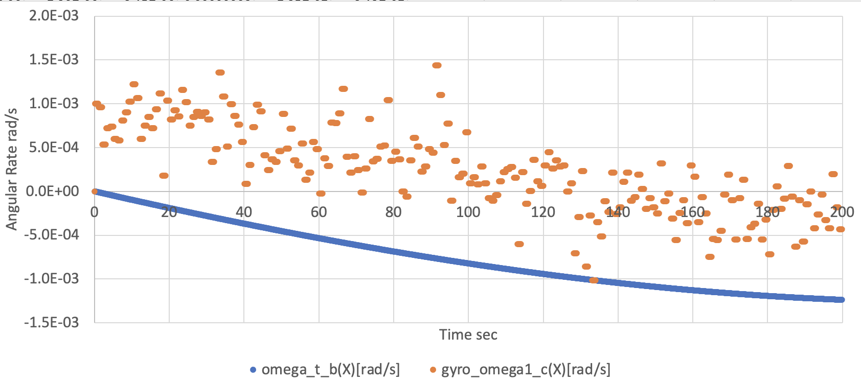
- We edited the file as
3. Add another Gyro sensor
- You can add multiple components in your
s2e-usersimulation case similar to the above sequence.
-
Open
user_components.hpp -
Add the following descriptions at the one line below of
GyroSensor *gyro_sensor_;GyroSensor *gyro_sensor_2_; //!< Gyro sensor 2 -
Open
user_components.cpp -
Edit the constructor function to add the following description to create the second instance of the GYRO class
file_name = iniAccess.ReadString("COMPONENT_FILES", "gyro_file_2"); configuration_->main_logger_->CopyFileToLogDirectory(file_name); gyro_sensor_2_ = new GyroSensor(InitGyroSensor(clock_generator, 2, file_name, compo_step_sec, dynamics)); -
Add the following descriptions at the one line below of
delete gyro_;in the destructordelete gyro_sensor_2_; -
Edit the
LogSetUpfunction as follows to register log outputvoid UserComponents::LogSetup(Logger &logger) { logger.AddLogList(gyro_sensor_); logger.AddLogList(gyro_sensor_2_); } -
Open
user_satellite.ini -
Add the following descriptions at the bottom line of
[COMPONENT_FILES]to set the initialize file for the gyro sensorgyro_file_2 = ../../data/initialize_files/components/gyro_sensor_yyy.ini -
Copy the
data/initialize_files/components/gyro_sensor_xxx.inifile and rename it asgyro_sensor_yyy.ini -
Edit
gyro_sensor_yyy.inito custom the noise performance of the second gyro sensor- Edit sensor ID like
[GYRO_SENSOR_1]to[GYRO_SENSOR_2] - Edit sensor ID like
[SENSOR_BASE_GYRO_SENSOR_1]to[SENSOR_BASE_GYRO_SENSOR_2]
- Edit sensor ID like
-
Build the
s2e-userand execute it -
Check the log output file to find
gyro_sensor2_measured_angular_velocity_c, the second gyro sensor's output angular velocity value in the component frame.
How To Make New Components
1. Overview
- In the How To Add Components tutorial, we have added existing components to the simulation scenario.
- This tutorial explains how to make a new component into the s2e-user directory.
- Note: You can move the source files for the new component into the s2e-core repository if the component is useful for all S2E users.
- The supported version of this document
- Please confirm that the version of the documents and s2e-core is compatible.
2. Overview of component expression in S2E
- Source codes emulating components are stored in the
s2e-core/src/componentsdirectory. - All components need to inherit the base class
Componentfor general functions of components, and most of the components also inherit the base classILoggablefor the log output function. Componentclass- The base class has an important virtual function
MainRoutine, and subclasses need to define it in their codes.- When an instance of the component class is created, the
MainRoutinefunction is registered in theTickToComponent, and it will be automatically executed in theSpacecraftclass. - The main features of the components such as observation, generate force, noise addition, communication, etc... should be written in this function.
- When an instance of the component class is created, the
PowerOffRoutineis also important especially for actuators. This function is called when the component power line is turned off. Users can stop force and torque generation and initialize the component states.
- The base class has an important virtual function
- Power related functions
SetPowerStateandGetCurrentare power related functions. If you want to emulate power consumption and switch control, you need to use the functions.
ILoggableclass- This base class has two important virtual functions
GetLogHeaderandGetLogValue, for CSV log output. - These functions are registered into the log output list when the components are added in
UserComponents::LogSetUp
- This base class has two important virtual functions
- Communication with OBC
- If users want to emulate the communication(telemetry and command) between the components and the OBC, they can use the base class
UartCommunicationWithObcorI2cTargetCommunicationWithObc. - These base classes also support a feature to execute HILS function.
- If users want to emulate the communication(telemetry and command) between the components and the OBC, they can use the base class
3. Make a simple clock sensor without initialize file
- This chapter explains how to make a simple clock sensor, which observes the simulation elapsed time with a bias noise.
- Users can find the sample codes in s2e-user-example/sample/how-to-make-new-components.
- The sample codes already including the initialize file for the
ClockSensor. Please edit the code a bit to learn the procedure step by step.
- The sample codes already including the initialize file for the
-
The
clock_sensor.cpp, .hppare created in thecomponentsdirectory.- The
ClockSensorclass counts clock with a constant bias noise. - The class inherits the
Componentand theILoggablebase classes as explained above.
- The
-
The
user_components.hppanduser_components.cppare edit similar procedure with the How To Add Components- The constructor of the
ClockSensorrequires arguments asprescaler,clock_generator,simulation_time, andbias_s. prescalerandbias_sare user setting parameters for the sensor, and you can freely set these values.clock_generatoris an argument for theComponentbase class.simulation_timeis a specific argument for theClockSensorto get true time information. TheSimulationTimeclass is managed in theGlobalEnvironment, and theGlobalEnvironmentis instantiated in theSimulationCaseclass.- We need to add the following codes to
user_components.cpp.- Instantiate the
ClockSensorin the constructor.
clock_sensor_ = new ClockSensor(10, clock_generator, global_environment->GetSimulationTime(), 0.001);- Delete the
clock_sensor_in the destructor.
delete clock_sensor_;- Add log set up into the
LogSetUpfunction.
logger.AddLogList(clock_sensor_); - Instantiate the
- The constructor of the
-
Build
s2e-userand execute it -
Check the log file to confirm the output of the
clock_sensor_observed_time[sec]- The output of the clock sensor has an offset error defined by the
bias_svalue, and the update frequency is decided by theprescalerand thecomponent_update_period_sin the base ini file.
- The output of the clock sensor has an offset error defined by the
4. Make an initialize file for the clock sensor
- Usually, we want to change the parameters of components such as noise properties, mounting coordinates, and others without rebuilding. So this section explains how to make an initialize file for the
ClockSensor.
-
The initialize function
InitClockSensoris defined in theclock_sensor.hpp.- The initialize function requires arguments as
clock_generator,simulation_time, andfile_name. clock_generatorandsimulation_timeare same argument with the constructor of theClockGenerator.file_nameis the file path to the initialize file for theClockSensor.
- The initialize function requires arguments as
-
Edit the
user_components.hppanduser_components.cppas followsuser_components.cpp- Edit making instance of the
clock_sensorat the constructor// Clock Sensor std::string file_name = iniAccess.ReadString("COMPONENT_FILES", "clock_sensor_file"); configuration_->main_logger_->CopyFileToLogDirectory(file_name); clock_sensor_ = new ClockSensor(InitClockSensor(clock_generator, global_environment->GetSimulationTime(), file_name));- The first line get the file path of the initialize file of the clock sensor.
- The second line copy the initialize file to the log output directory to save the simulation setting.
- The third line make the instance of the
ClockSensor.
- Edit making instance of the
-
Make
clock_sensor.iniintos2e-user/data/initialize_files/componentsfrom./Tutorial/SampleCodes/clock_sensor -
Edit
user_satellite.inito add the following line at the [COMPONENT_FILES] section of the fileclock_sensor_file = INI_FILE_DIR_FROM_EXE/components/clock_sensor.ini- The keyword
INI_FILE_DIR_FROM_EXEis defined in theCMakeList.txtto handle the relative path to the initialize files.
- The keyword
-
Build
s2e-userand execute it -
Check the log file
-
Edit the
clock_sensor.iniand rerun thes2e-userto confirm the initialize file can affect the result.
How To Use Monte Carlo Simulation
1. Overview
- S2E has a framework to execute the Monte Carlo Simulation.
- The feature provides a framework to randomize arbitrary parameters in each class.
- Users can set the mean value and standard deviation for the randomized parameters with
simulation_base.inifile of each user.- Please see the specification document for Monte Carlo Simulation for a detailed description.
- This tutorial explains how to randomly change the initial value of the spacecraft angular velocity.
- There are sample codes in s2e-user-example/sample/how-to-use-monte-carlo-simulation.
- The supported version of this document
- Please confirm that the version of the documents and s2e-core is compatible.
2. Edit Simulation Case
- To use the Monte Carlo simulation, users have to edit their
user_case.hppanduser_case.cpp user_case.hpp- Add header including
#include <./simulation/monte_carlo_simulation/monte_carlo_simulation_executor.hpp> - Add private member variables for
MonteCarloSimulationExecutor.MonteCarloSimulationExecutor &monte_carlo_simulator_; - Replace the constructor of UserCase class to add arguments for Monte Carlo simulation.
UserCase(const std::string initialize_base_file, MonteCarloSimulationExecutor &monte_carlo_simulator, const std::string log_path);
- Add header including
user_case.cpp- Add header including
#include <./simulation/monte_carlo_simulation/simulation_object.hpp> - Replace the constructor as follows
UserCase::UserCase(const std::string initialize_base_file, MonteCarloSimulationExecutor &monte_carlo_simulator, const std::string log_path) : SimulationCase(initialize_base_file, monte_carlo_simulator, log_path), monte_carlo_simulator_(monte_carlo_simulator) {} - Edit
InitializeTargetObjectsfunction- Edit log file name definition and
- Add
MonteCarloSimulationExecutorinitialization// Monte Carlo Simulation monte_carlo_simulator_.SetSeed(); monte_carlo_simulator_.RandomizeAllParameters(); SimulationObject::SetAllParameters(monte_carlo_simulator_); monte_carlo_simulator_.AtTheBeginningOfEachCase();
- Add log settings for the Monte Carlo simulation
- The
GetLogHeaderandGetLogValuefunctions are used for Monte Carlo log output.- The log output defined in the function is executed at the beginning and end of a simulation case.
- The output line will be
2N+1, where N is the sample number of the Monte Carlo simulation.- +1 line is for headers.
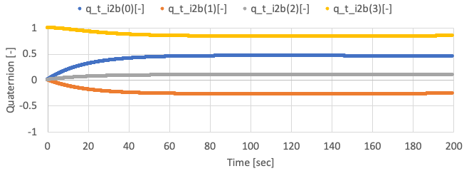
- In this tutorial, time, angular velocity, and quaternion are logged.
- Users can customize this output depending on their needs.
std::string UserCase::GetLogHeader() const
{
  std::string str_tmp = "";

  str_tmp += WriteScalar("elapsed_time", "s");
  str_tmp += WriteVector("spacecraft_angular_velocity", "b", "rad/s", 3);
  str_tmp += WriteVector("spacecraft_quaternion", "i2b", "-", 4);

  return str_tmp;
}
std::string UserCase::GetLogValue() const
{
  std::string str_tmp = "";

  str_tmp += WriteScalar(global_environment_->GetSimulationTime().GetElapsedTime_s());
  str_tmp += WriteVector(spacecraft_->GetDynamics().GetAttitude().GetAngularVelocity_b_rad_s(), 3);
  str_tmp += WriteQuaternion(spacecraft_->GetDynamics().GetAttitude().GetQuaternion_i2b());

  return str_tmp;
}
- The
- Add header including
3. Edit s2e_user.cpp code
- To use the Monte Carlo Simulator, users have to edit their
s2e_user.cpp - Add header file
#include <./simulation/monte_carlo_simulation/initialize_monte_carlo_simulation.hpp> - If you find description below
rewrite as the following description#include "library/logger/logger.hpp"#include "library/logger/initialize_log.hpp" - Make an instance of
MonteCarloSimulatorExecutorand Logger for Monte Carlo logMonteCarloSimulationExecutor *mc_simulator = InitMonteCarloSimulation(ini_file); Logger *log_mc_sim = InitMonteCarloLog(ini_file, mc_simulator->IsEnabled()); - Add while loop for Monte Carlo simulation as follows
while (mc_simulator->WillExecuteNextCase()) {
  auto simulation_case = UserCase(ini_file, *mc_simulator);
  // Initialize
  log_mc_simulator->AddLogList(&simulation_case);
  if (mc_simulator->GetNumberOfExecutionsDone() == 0) log_mc_simulator->WriteHeaders();
  simulation_case.Initialize();
  // Main
  log_mc_simulator->WriteValues();  // log initial value
  simulation_case.Main();
  mc_simulator->AtTheEndOfEachCase();
  log_mc_simulator->WriteValues();  // log final value
  log_mc_simulator->ClearLogList();
}

delete log_mc_simulator;
delete mc_simulator;
4. Initialize file for Monte Carlo simulator
-
Edit
user_simulation_base.inito add the following description[MONTE_CARLO_EXECUTION] // Whether Monte-Carlo Simulation is executed or not monte_carlo_enable = ENABLE // Whether you want output the log file for each step log_enable = ENABLE // Number of execution number_of_executions = 3 [MONTE_CARLO_RANDOMIZATION] parameter(0) = attitude0.angular_velocity_b_rad_s attitude0.angular_velocity_b_rad_s.randomization_type = CartesianUniform attitude0.angular_velocity_b_rad_s.mean_or_min(0) = 0.0 attitude0.angular_velocity_b_rad_s.mean_or_min(1) = 0.0 attitude0.angular_velocity_b_rad_s.mean_or_min(2) = 0.0 attitude0.angular_velocity_b_rad_s.sigma_or_max(0) = 0.05817764 // 3-sigma = 10 [deg/s] attitude0.angular_velocity_b_rad_s.sigma_or_max(1) = 0.05817764 // 3-sigma = 10 [deg/s] attitude0.angular_velocity_b_rad_s.sigma_or_max(2) = 0.05817764 // 3-sigma = 10 [deg/s] -
You can set the following parameters
monte_carlo_enable:ENABLE: S2E executes the Monte Carlo Simulation.DISABLE: S2E executes a simulation case defined in ini files.
log_enable:ENABLE: A default csv log file is outputted for each sample case.- Note: 100 csv files will be generated when you set
number_of_executions = 100.
- Note: 100 csv files will be generated when you set
DISABLE: No default csv log file will be generated. Only amonte_carlo csv logfile will be generated.- Note: When
monte_carlo_enable = DISABLE, a default csv log file will always be generated.
- Note: When
number_of_executions: integer lager than 1- The total calculation time is proportional to this value.
-
Randomized parameters
- randomization_type: You can choose the randomization type. See Monte Carlo Simulation for detail.
mean_or_min: Input mean value or minimum value. (Depends on Randomization type)sigma_or_max: Input standard deviation or maximum value. (Depends on Randomization type)
6. Execute and check logs
- Build the
S2E_USERand execute it. - In the
datadirectory, you can find onexxxx_monte_carlo.csvfile and severalxxxx_default.csvfiles, which depend on your Monte Carlo Simulator setting. - The initial value of angular velocity is randomly varied by the Monte Carlo Simulator.
How To Add Control Algorithms
1. Overview
- In the How To Make New Components tutorial, we have newly made components emulating codes and adding the new components into our simulation scenario.
- Now we can simulate the behavior of spacecraft free motion and emulate the behavior of sensors and actuators.
- This tutorial explains how to add a Control Algorithm to the simulation scenario.
- For a practical satellite project, we should implement the control algorithm as actual flight software like C2A into the S2E. However, using actual flight software is usually overdoing for use cases such as research and the initial phase of satellite projects.
- So, we introduce the following three methods, and users can choose a suitable method.
Direct method: Directly control physical quantity without sensors, actuators, and their noises- For theoretical research and preliminary analysis for satellite projects
Component method: Control using sensors and actuators without flight S/W framework- We can include sensing and actuation noise.
- For engineering research and preliminary analysis for satellite projects
- From v6.0.0, we have
idealandrealdirectories in thes2e-core/src/components. Users can useidealcomponents for the early stage of the analysis and can userealcomponents for more detailed analysis. Mixing these components is also possible.
Flight S/W method: Control using sensors and actuators with flight S/W framework- For actual satellite projects
- The supported version of this document
- Please confirm that the version of the documents and s2e-core are compatible.
2. Direct method
- This chapter introduces how to add a control algorithm without sensors and actuators.
- This method directly measures the satellite's physical quantity and generates torque and force acting on the satellite.
- To do that, users need to edit the
Updatefunction in theUserSat.cpp.- A sample code is in s2e-user-example/sample/how-to-add-control-algorithm-direct-method
- The
UserSatelliteclass already has satellite attitude, orbit, and local environment information since it inherits theSpacecraftbase class. So users can easily access these values. - To measure physical quantities, users can use getter functions defined in the
Attitude,Orbit, andLocalEnvironmentclasses asdynamics_->GetAttitude().GetAngularVelocity_b_rad_s(). - To generate torque and force, users can use
dynamics_->AddTorque_b_Nmanddynamics_->AddForce_b_N. - The sample codes are in
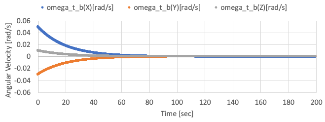
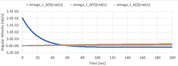
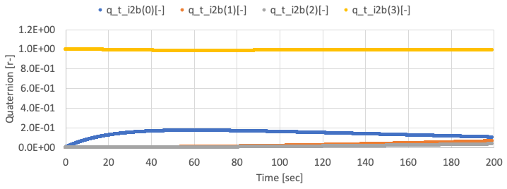
SampleCodes/control_algorithm/direct_method/user_satellite.cpp, and you can see very simple detumbling with the proportional control method. - By using the sample code with initial angular velocity = [0.05, -0.03, 0.01] rad/s, the following results are given.
-
You need to edit the initialize file to set the initial angular velocity.
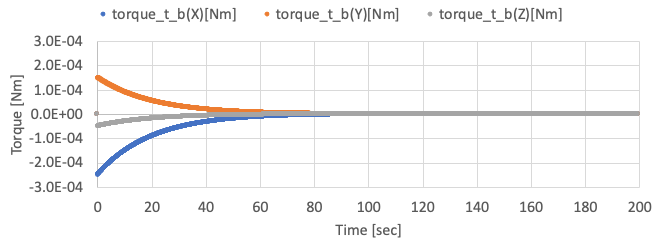
-
3. Component method: Using ideal components
- TBW
- Users can refer the s2e-ff as an example of the ideal component method.
4. Component method: Using real components
- This chapter introduces a method to add a control algorithm using realistic sensors and actuators. - This method measures a satellite's physical quantity via sensors, generates torque and force via actuators, and executes control algorithms on OBC.
- This tutorial assumes the spacecraft has a three-axis gyro sensor, a reaction wheel, and an OBC.
- The sample codes are in s2e-user-example/sample/how-to-add-control-algorithm-using-real-component.
- Firstly, users need to make the
UserOnBoardComputerclass to emulate the OBC.- Copy the
user_on_board_computerfiles to thes2e-user/src/componentsfrom thecomponent_method/src/components, and add theuser_on_board_computer.cppto theset(SOURCE_FILES)in theCMakeLists.txtto compile it. - The
UserOnBoardComputerclass has theUserComponentsclass as a member, and users can access all components to get sensing information or set the output of actuators. - In this tutorial, the angular velocity is measured by the gyro sensor. After that RW's output torque is calculated using the X-axis of the measured angular velocity, and the torque is set to RW.
- Copy the
- Next, users need to add the
UserOnBoardComputerinto theUserComponentsclass. You can copy theuser_componentsfiles to thes2e-user/src/simulation/spacecraftfrom thecomponent_method/src/simulation. - Finally, users need to add new source codes to the
CMakeLists.txtto compile them.- You have to add
reaction_wheel_xxx.initos2e-user/data/initialize_files/components - Refer to
SampleCodes/control_algorithm/component_method/data/reaction_wheel_xxx.iniif necessary.
- You have to add
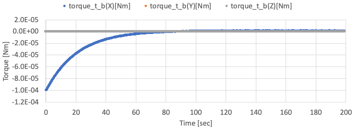
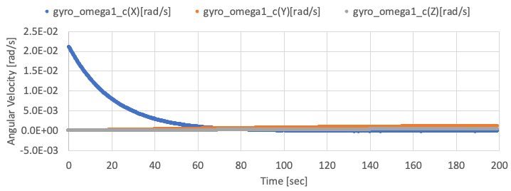
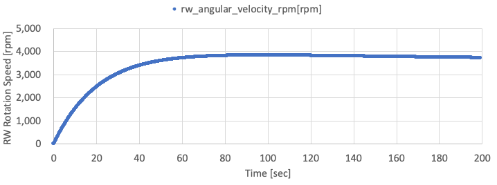
- By using the sample code, the following results are given.
-
The X-axis angular velocity is controlled, but other axes are not controlled well since the satellite only has an RW on X-axis. The X-axis angular velocity has offset value since the gyro has offset noise.
-
The following two figure shows the observed angular velocity by gyro and the rotation speed of the RW. You can find the observed X-axis angular velocity reaches zero by the control.
-
5. FlightSW method: Control algorithm within C2A
- TBW
- Users can refer the s2e-aobc as an example of the flight software method.
How to integrate C2A
1. Overview
- C2A (Command Centric Architecture) is an architecture for spacecraft flight software developed by ISSL.
- S2E can execute C2A as flight software for onboard algorithm development and debugging.
- This document describes how to integrate the C2A within S2E.
- Notes
- C2A is written in C language, but S2E builds C2A as C++.
- The supported version of this document
- Please confirm that the version of the documents and s2e-core are compatible.
2. Overview of C2A execution in S2E
- Directory Construction
- Make
FlightSWdirectory at same directory withs2e-coreands2e-user. - Make a
c2a-userdirectory inFlightSWand set the C2A source code you want to use.├─ FlightSW │ └─ c2a-user │ └─ src_user │ └─ src_core └─ s2e-user-example ├─ s2e-core └─ ExtLibraries - Edit
s2e-user/CMakeLists.txtas follows.set(C2A_NAME "c2a_oss")- Edit the directory name
c2a_ossaccording to your situation. - In the case of the above directory structure, you need to edit as
c2a-user
- Edit the directory name
option(USE_C2A "Use C2A" OFF)- Turn on the
USE_C2Aflag asoption(USE_C2A "Use C2A" ON)
- Turn on the
- Make
- Notes
- In the default setting of S2E, C2A is built but isn't executed. To execute the C2A, users need to add an onboard computer, which can execute the C2A.
- The
s2e-corehas the ObcWithC2a class as a component, and users can use it to execute the C2A. - Users can use the
ObcWithC2aclass in theUserComponentsclass, the same as other components.
- Build the
s2e_user- Note: When you add new source files in the C2A, you need to modify the
c2a-user/CMakeLists.txtto compile them in the S2E. - Users can choose the construction of CMake as users need. For example, the sample codes have several
CMakeLists.txtfiles in each directory to set the compile targets, so users need to modify them to add the target source codes.
- Note: When you add new source files in the C2A, you need to modify the
3. How to build C2A in S2E with the sample codes
-
Sample codes
- A sample of s2e-user: s2e-user-example/sample/how-to-integrate-c2a
- A sample of c2a-user: C2A minimum user in
c2a-core.
-
Preparing development environment
-
Clone the
s2e-user-exampleand switch the branch tosample/how-to-integrate-c2a. -
Make
FlightSWdirectory at same directory withs2e-core. -
Clone
c2a-core v3.8.0in theFlightSWdirectory. -
Execute setup script
- Mac or Linux Users:
c2a-core/setup.sh - Windows Users:
c2a-core/setup.bat
- Mac or Linux Users:
-
Open
s2e-user-for-c2a-core/CMakeLists.txtand editset(C2A_NAME "c2a_sample")toset(C2A_NAME "c2a-core/Examples/minimum_user") -
For users who don't use Windows
- open
c2a-core/Examples/minimum_user/CMakeLists.txtand editoption(USE_SCI_COM_WINGS "Use SCI_COM_WINGS" ON)tooption(USE_SCI_COM_WINGS "Use SCI_COM_WINGS" OFF) - This setting turns off the feature to communicate with WINGS ground station. Currently, this feature is available only for Windows users.
- open
-
Please check the following directory construction
├─ FlightSW │ └─ c2a-core │ └─ Examples │ └─ minimum_user └─ s2e-user-example ├─ s2e-core └─ ExtLibraries -
Build and execute the
s2e-user-example. -
Users can see the following output in a terminal. The
CYCLE: TOTALvalue is incremented.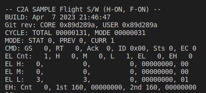
-
4. Communication between C2A and S2E for SILS test
- Generally, communication between flight software and S2E is executed via
OnBoardComputerclass. - The
OnBoardComputerclass has communication ports and communication functions. Other components and flight software can use the communication functions to communicate each other. - For C2A, the
ObcWithC2ahas the following functions for C2A flight software. The driver functions in the flight software can use these functions. It is essential to use the sameport_idwith the component setting in S2E. The details are described in specification documents for each feature.- Serial communication functions
int OBC_C2A_SendFromObc(int port_id, unsigned char* buffer, int offset, int count); int OBC_C2A_ReceivedByObc(int port_id, unsigned char* buffer, int offset, int count); - I2C communication functions
int OBC_C2A_I2cWriteCommand(int port_id, const unsigned char i2c_addr, const unsigned char* data, const unsigned char len); int OBC_C2A_I2cWriteRegister(int port_id, const unsigned char i2c_addr, const unsigned char* data, const unsigned char len); int OBC_C2A_I2cReadRegister(int port_id, const unsigned char i2c_addr, unsigned char* data, const unsigned char len); - GPIO
int OBC_C2A_GpioWrite(int port_id, const bool is_high);
bool OBC_C2A_GpioRead(int port_id);
- Serial communication functions
- Currently, the C2A uses the wrapper functions in IfWrapper/Sils. The functions automatically overload the normal IfWrapper functions when C2A is executed on the S2E.
- Other interfaces like SPI, etc., will be implemented.
5. Example of S2E-C2A communication
-
This section shows an example of communication between a component in S2E and an application in C2A.
-
The sample codes
-
Preparation
- See
Ch. 3 How to build C2A in S2E with the sample codes.
- See
-
Modification of the S2E side
- Users can use the ExampleSerialCommunicationWithObc class in
s2e-coreas a test component to communicate with C2A. - Please refer the sample codes in s2e-user-example/sample/how-to-integrate-c2a.
- Add
ExampleSerialCommunicationWithObcas a component inuser_components.cpp and .hpp.- In this example, the
ObcWithC2ais executed as 1kHz, and theExampleSerialCommunicationWithObcis executed as 1Hz.
- In this example, the
- Users can use the ExampleSerialCommunicationWithObc class in
-
Modification of the C2A side
- Please refer the sample codes in
Tutorials/SampleCodes/c2a_integration/c2a_src_user.- The directory structure of
c2a_src_useris the same with that ofc2a-core/Examples/minimum_user/src/src_user.
- The directory structure of
- We need to add a new driver instance application to communicate with the
ExampleSerialCommunicationWithObccomponent.- Copy
Application/DriverInstances/di_s2e_uart_test.c and .h - Edit
CMakeLists.txtin the Application directory to adddi_s2e_uart_test.cas a compile target.
- Copy
- Edit
app_registry.c, handapp_headers.hin theApplicationdirectory to register the applications ofdi_s2e_uart_test.- We have two applications
AR_DI_S2E_UART_TESTandAR_DI_DBG_S2E_UART_TEST.
- We have two applications
- Edit
Setting/Modes/TaskLists/Elements/tl_elem_drivers_update.cto add theAR_DI_S2E_UART_TESTto execute the application in the tasklist. - Edit
Setting/Modes/TaskLists/Elements/tl_elem_debug_display.cto add theAR_DI_DBG_S2E_UART_TESTto execute the application in the tasklist.
- Please refer the sample codes in
-
Execution and Result
-
The C2A's
AR_DI_S2E_UART_TESTapplication sends characters to the S2E'sExampleSerialCommunicationWithObccomponent likeSETA, SETB, SETC, ..., SETZ, SETA -
The
ExampleSerialCommunicationWithObccomponent receives the characters and stores the set characters likeA, B, C, ..., Z, A -
The
ExampleSerialCommunicationWithObccomponent sends the stored characters as telemetry likeA, BA, CBA, ..., ZYX -
The
AR_DI_S2E_UART_TESTapplication receives the telemetry, and theAR_DI_DBG_S2E_UART_TESTapplication prints the first three characters in the debug output console like the following figure.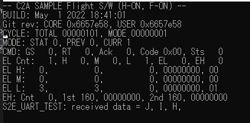
-
How to Perform UART HILS Test
1. Overview
- Using the SerialPort Class in System.IO.Ports Namespace, you can perform serial communication from the COM port of your computer.
- The HILS test can be performed by replacing satellite components with simulated components in S2E.
- This document describes how to perform HILS Test with UART components.
- If you want to perform HILS Test with I2C components, refer to here.
2. How to build files for the HILS test
- Currently, the HILS test is only available for Visual Studio users on Windows.
- Serial port operations are written in
Interface/HilsInOut/Ports/HilsUartPort.cppin c++/cli language. - When users want to execute the HILS test, complete the following steps.
-
Edit
s2e-core/CMakeLists.txtoption(USE_HILS "Use HILS" OFF)->option(USE_HILS "Use HILS" ON)
-
build
s2e-core
-
- Note: Currently, breakpoints do not work if you build c++/cli and c++ files simultaneously.
3. Sample codes for UART communication
-
The supported version of this document
- Please confirm that the version of the documents and s2e-core is compatible.
-
Hardware Settings
- Set loopback connection of two USB-UART converters using two USB ports of your computer.
- Check the COM port number for each connection.
- This tutorial assumes the use of USB-COMi-SI, a USB-UART converter.
-
Software Settings
s2e-core/src/Component/Abstract/ExpHils.cppis an example of a simulation component for serial port communication.ExpHilsis instantiated ins2e-core/src/Simulation/Spacecraft/SampleComponents.cpp.- Uncomment as follows in
s2e-core/src/Simulation/Spacecraft/SampleComponents.cpp.// UART tutorial. Comment out when not in use. exp_hils_uart_responder_ = new ExpHils(clock_gen, 1, obc_, 3, 9600, hils_port_manager_, 1); exp_hils_uart_sender_ = new ExpHils(clock_gen, 0, obc_, 4, 9600, hils_port_manager_, 0);delete exp_hils_uart_responder_; delete exp_hils_uart_sender_;- Edit the constructor's argument based on the COM port number checked above.
- The fourth argument of ExpHils constructor is COM port number.
- Edit the constructor's argument based on the COM port number checked above.
- Uncomment as follows in
s2e-core/src/Simulation/Spacecraft/SampleComponents.h.ExpHils* exp_hils_uart_responder_; ExpHils* exp_hils_uart_sender_; - For the HILS test, edit the setting of simulation speed in
s2e-core/data/SampleSat/ini/SampleSimBase.ini.// Simulation speed. 0: as fast as possible, 1: real-time, >1: faster than real-time, <1: slower than real-time SimulationSpeed = 1
-
Execution and Result
- There are two ExpHils components, a sender component and a responder component.
- The sender component sends out a new message like
ABC,BCD, .... - The responder component returns the message as received.
- Data returned from the responder to the sender is output to the console.
- The sender component sends out a new message like
- If the comment
Error: the specified step_sec is too small for this computer.appears, setStepTimeSecin SampleSimBase.ini to a larger value.
- There are two ExpHils components, a sender component and a responder component.
How to Perform I2C HILS Test
1. Overview
- Using the SerialPort Class in System.IO.Ports Namespace, you can perform serial communication from the COM port of your computer.
- The HILS test can be performed by replacing satellite components with simulated components in S2E.
- This document describes how to perform HILS Test with I2C components.
- If you want to perform HILS Test with UART components, refer to here.
2. How to build files for the HILS test
- Currently, the HILS test is only available for Visual Studio users on Windows.
- Serial port operations are written in
Interface/HilsInOut/Ports/HilsUartPort.cppin c++/cli language. - When users want to execute the HILS test, complete the following steps.
- Edit
s2e-core/CMakeLists.txtoption(USE_HILS "Use HILS" OFF)->option(USE_HILS "Use HILS" ON)
- build
s2e-core
- Edit
- Note: Currently, breakpoints do not work if you build c++/cli and c++ files simultaneously.
3. Sample codes for I2C communication
-
The SerialPort class can also be used to perform HILS tests on simulated I2C components. It is assumed that USB-I2C converters will be used and that serial communication will be performed between the COM port and the converter.
-
The supported version of this document
- Please confirm that the version of the documents and s2e-core is compatible.
-
Hardware Settings
- Set loopback connection of a USB-I2C controller converter and a USB-I2C target converter using two USB ports of your computer.
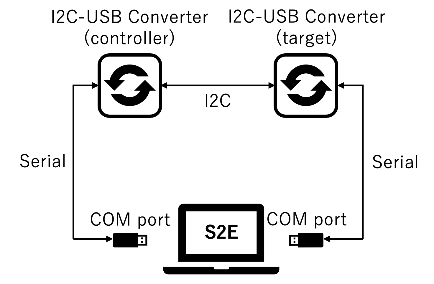
- Check the COM port number for each connection.
- This tutorial assumes the use of SC18IM700, a USB-I2C Controller converter and MFT200XD, a USB-I2C Target converter.
- Note Loopback is not always necessary. Only one of the I2C controller or the I2C target can be simulated in S2E. In a general HILS configuration, the I2C controller is an OBC. s2e-core provides a simulated component of the I2C controller in order to validate the simulated component of the I2C target.
- Set loopback connection of a USB-I2C controller converter and a USB-I2C target converter using two USB ports of your computer.
-
Software Settings
s2e-core/src/Component/Abstract/ExpHilsI2cController.cppands2e-core/src/Component/Abstract/ExpHilsI2cTarget.cppare examples of simulation components for I2C communication.ExpHilsI2cControllerandExpHilsI2cTargetare instantiated ins2e-core/src/Simulation/Spacecraft/SampleComponents.cpp.- Uncomment as follows in
s2e-core/src/Simulation/Spacecraft/SampleComponents.cpp.// I2C tutorial. Comment out when not in use. exp_hils_i2c_controller_ = new ExpHilsI2cController( 30, clock_gen, 5, 115200, 256, 256, hils_port_manager_); exp_hils_i2c_target_ = new ExpHilsI2cTarget(1, clock_gen, 0, 0x44, obc_, 6, hils_port_manager_);delete exp_hils_i2c_controller_; delete exp_hils_i2c_target_;- Edit the constructor's argument based on the COM port number checked above.
- The third argument of ExpHilsI2cController constructor and the sixth argument of ExpHilsI2cTarget constructor are COM port numbers.
- Edit the baud rate and I2C address according to the converter and simulation conditions.
- The baud rate is specified by the fourth argument of the ExpHilsI2cController constructor and the I2C address by the fourth argument of the ExpHilsI2cTarget constructor.
- Edit the constructor's argument based on the COM port number checked above.
- Uncomment as follows in
s2e-core/src/Simulation/Spacecraft/SampleComponents.h.ExpHilsI2cController* exp_hils_i2c_controller_; ExpHilsI2cTarget* exp_hils_i2c_target_; - If necessary, modify ExpHilsI2cController and ExpHilsI2cTarget files to adjust to the converter.
- For the HILS test, edit the setting of simulation speed in
s2e-core/data/SampleSat/ini/SampleSimBase.ini.// Simulation speed. 0: as fast as possible, 1: real-time, >1: faster than real-time, <1: slower than real-time SimulationSpeed = 1
-
Execution and Result
- There are two components, an I2C controller component and an I2C target component.
- I2C controller
- Send a command to the I2C target.
- Send a command to request a telemetry. 1 byte register address is sent to specify the first address of the data to be read from the I2C controller.
- Send a command to read a telemetry from the USB-I2C target converter.
- Send a command to the I2C target.
- I2C target
- Receive commands from the I2C controller and send telemetry to the I2C controller.
- After receiving the telemetry request command, send the telemetry (like ABCDE, BCDEF, ...) to the USB-I2C target converter.
- Receive commands from the I2C controller and send telemetry to the I2C controller.
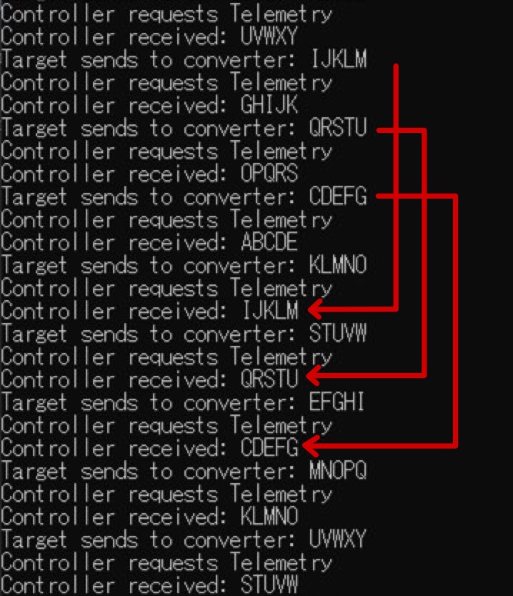
- Note Currently, the latency from the time the USB-I2C target converter receives the data via I2C communication to the time it is sent to the I2C target component via serial communication is too long, at least 1ms, making it impossible to immediately respond to telemetry request commands.
- Three frames of telemetry are stored in the USB-I2C target converter in advance.
- Each time the I2C controller reads the telemetry stored in the USB-I2C target converter, the I2C target component adds the telemetry to the USB-I2C target converter.
- The data sent by the I2C target and the data received by the I2C controller are the outputs to the console. Since there are three frames accumulated in the USB-I2C target converter, the I2C controller receives telemetry sent three cycles before from the I2C target.
- If the comment
Error: the specified step_sec is too small for this computer.appears, setStepTimeSecin SampleSimBase.ini to a larger value.
How to simulate multiple satellites
1. Overview
- S2E can simulate multiple satellites.
- This document describes how to simulate multiple satellites.
- For the sample codes, please see s2e-user-example/sample/how-to-simulate-multiple-satellites.
- The supported version of this document
- Please confirm that the version of the documents and s2e-core are compatible.
2. How to add a new satellite
-
Edit
inifiles- Add
inifiles for the new satellite.satellite.ini,disturbance.ini,local_environment.ini,structure.iniare needed.
- Register the
inifile for the new satellite insimulation_base.ini- The arguments of
satellite_fileare used as satellite ID in simulation.[SIMULATION_SETTINGS] number_of_simulated_spacecraft = 2 spacecraft_file(0) = INI_FILE_DIR_FROM_EXE/user_satellite.ini spacecraft_file(1) = INI_FILE_DIR_FROM_EXE/user_satellite2.ini
- The arguments of
- Add
-
Edit source code
-
Add new
UserSatelliteinstances toCasemembers inuser_case.hpp.UserSatellite *spacecraft0_; //!< Instance of spacecraft UserSatellite *spacecraft1_; //!< Instance of spacecraft -
Edit
user_case.cppto copy the spacecraft related codes as the sample code.- Please see the sample code for more details.
-
-
Build and execute the
s2e-user -
You can see the log
spacecraft_angular_velocity_b_x[rad/s]twice. The first one is the angular velocity ofsatellite 0, and the second one is the angular velocity ofsatellite 1in the log file.
3. Advanced usage
- In the sample, the
satellite0_and thesatellite1_are completely the same, but users can change the settings of these satellites with editing theinifiles.- Users can change the orbit, initial attitude, satellite structure and so on.
- Users also can set the different components for the
satellite0 and 1, when users define differentUserSatelliteandUserComponentsclasses. - The document to use
relative informationwill be written. - Users can also refer the S2E-FF repository.
Overall Structure of S2E
1. Overview
- This document explains the overall structure of the S2E.
2. Structure of S2E
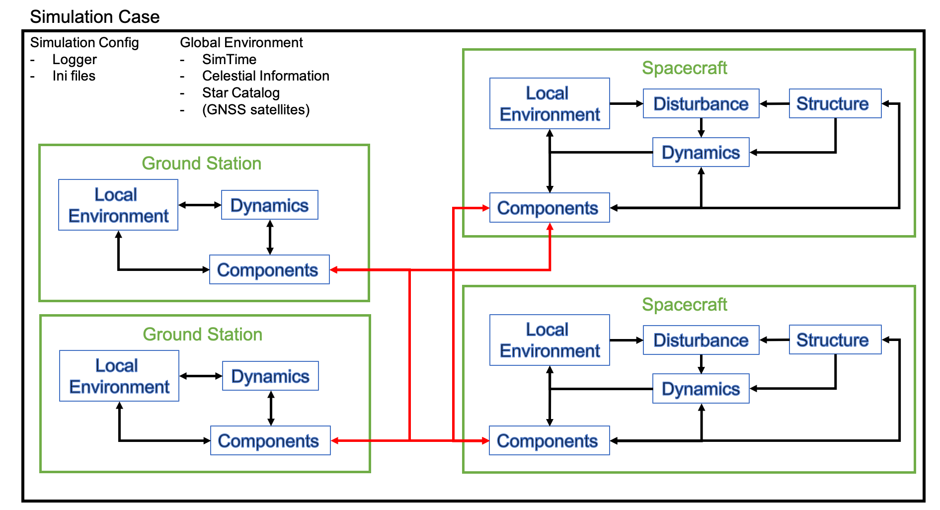
- The following figure shows the structure of the S2E.
2.1. Simulation Case
- The highest layer of the structure of S2E is the
Simulation Case, which is defined in thesrc/simulation/case/simulation_case.cpp. - The
Simulation Casealways hasSimulation ConfigurationandGlobal Environment.Simulation Configurationhas basic information on the interface of the simulation, such aslog outputandinitialize inputinformation.Global Environmentis defined as the common environment for the whole simulation case. It includes time, celestial information, star catalog, and GNSS satellite position.
- Users can make their
Simulation Caseby inheriting theSimulation Casebase class and adding simulation target objects (e.g., spacecraft and ground station) for their demand. - The defined simulation objects can use the information of
Simulation ConfigurationandGlobal Environment.
2.2. Spacecraft
- An essential simulation object is the
Spacecraftclass. Spacecraftclass has the following features to simulate the behavior of spacecraft in space.Structure- This class handles the structure information of the spacecraft, such as the mass, the inertia tensor, surface information, and residual magnetic moment.
- The information is used to calculate disturbance and propagate dynamics.
LocalEnvironment- This class handles space environment information around the spacecraft, such as air density, magnetic field, solar energy, and eclipse.
- The information is used to calculate disturbance and emulate environment sensors.
Disturbance- This class handles disturbances forces(accelerations) and torques.
- The information is used to propagate dynamics.
Dynamics- This class handles dynamics calculation for attitude, orbit, and thermal.
- This is the core of the numerical simulation.
Components- This class emulates the behavior of components mounted on the spacecraft. The spacecraft can measure the physical quantities and generate control output by using the components.
- This class is not defined in the Spacecraft base class, and users have to define it themselves.
- Users can add multiple spacecraft into their
SimulationCase, and these spacecraft can communicate via communication components.
2.3. Ground Station
- TBW
2.4. Structure of initializing files
- The structure of the initializing files follows the above figure.
simulation_base.inisets the parameters forSimulationCase, and file paths to each simulation object.satellite.inisets the parameters forSpacecraftand file paths to each component.
3. Structure of spacecraft components
Note: the structure of components is implemented now. So the following figure is just an idea, and it may be modified.
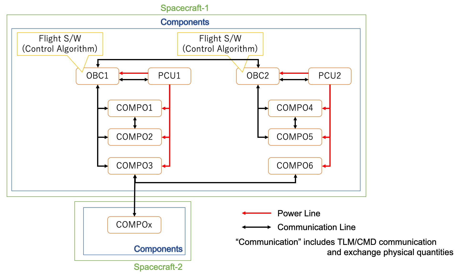 - Each component can communicate with other components.
- All components have a power wire, and power control components control the switch.
- Each component can communicate with other components.
- All components have a power wire, and power control components control the switch.
Specification of Component class
1. Overview
1. Functions
- The
Componentclass is an abstract class to handle the electrical power and the update timing of components. - This class has two virtual functions:
MainRoutineandFastUpdate. Both are called periodically. Users can select the functions according to the required calling period.- The
MainRoutinefunction is the components' main function. Most of the processing is handled in this function. - The
FastUpdatefunction handles the processes that need to be computed in a high-speed cycle. So, users will use this function only when high-frequency disturbances need to be calculated (e.g., RW jitter).
- The
2. Related Files
- Main file:
component.hpp,component.cpp
3. How to use
- Inherit this class by the user's component class.
- The
ReactionWheelinS2E_COREis useful as a usage example of theFastUpdate.
2. Explanation of Algorithm
1. Constructor
1. overview
- Users can set component update
prescalerand power port.
2. inputs
prescalerprescalerdetermines the execution cycle of theMainRoutinefunction.- The period of
MainRoutineequals toSimTime::compo_update_interval_sec$\times$prescaler.
clock_genclock_genis an instance that simulates the clock of a component.- Users do not need to care about this.
power_portpower_portis an instance that simulates the power supply
fast_prescalerfast_prescalerdetermines the execution cycle of theFastUpdatefunction.- The period of
FastUpdateequals toSimTime::compo_update_interval_sec$\times$fast_prescaler. - If you don't need to use
FastUpdate, you don't need to specify this (it is set to 1 by default).
3. algorithm
- N/A
4. note
- N/A
2. MainRoutine
1. overview
- Components' main function
2. inputs
time_counttime_countis incremented each time theTickfunction is called.- Users can use this timing information when they need for their components.
3. algorithm
- N/A
4. note
- All the components have to override the
MainRoutinefunction.
3. FastUpdate
1. overview
- This function handles the processes that need to be computed in a high-speed cycle.
2. inputs
- N/A
3. algorithm
- N/A
4. note
FastUpdatefunction is not a pure virtual function, so components without fast calculation do not need to override this function.- As explained in the
FastTicksection,ITickable::needs_fast_update_flag must be true to callFastUpdate. So, if users want to useFastUpdate, callITickable::SetNeedsFastUpdate(true)in the constructor of each component.
4. Tick
1. overview
- This function executes
MainRoutine. ClockGeneratorclass calls this function.
2. inputs
countcountis incremented each time theTickfunction is called.
3. algorithm
- Execute
MainRoutinewhen thecountis divisible by theprescaler. By this mechanism, the execution period ofMainRoutineis divided.
4. note
- N/A
5. FastTick
1. overview
- This function executes
FastUpdate. ClockGeneratorclass calls this function.
2. inputs
countcountis incremented each time theFastTickfunction is called.
3. algorithm
- Execute
FastUpdatewhen thecountis divisible by thefast_prescaler. By this mechanism, the execution period ofFastUpdateis divided.
4. note
ITickable::needs_fast_update_flag must be true to callFastUpdate. So, if you want to useFastUpdate, callITickable::SetNeedsFastUpdate(true)in the constructor of each component.
3. Results of verifications
- N/A
4. References
- N/A
Specification of UartCommunicationWithObc class
1. Overview
1. Functions
- The
UartCommunicationWithObcclass is an abstract class to communicate withOnBoardComputer. - Component classes can use this abstract class to emulate telemetry/command communication with an
OnBoardComputer. - This class also supports communication with
C2Ain theObcWithC2aclass.
2. Related files
- on_board_computer.cpp, hpp
- example_serial_communication_with_obc.cpp, hpp
- Users can find an example of using this class.
3. How to use
- Inherit this class by component class.
- Users need to set
sils_port_idand targetOnBoardComputerfor the communication.
- Users need to set
- This class has the following protected functions for telemetry/command communication. Users can call these functions in the
MainRoutineof the component.int ReceiveCommand(const int offset, const int rec_size); int SendTelemetry(const int offset); - In the protected functions, the following pure virtual functions are called. Users need to define the functions in the subclass.
virtual int ParseCommand(const int cmd_size)=0;
virtual int GenerateTelemetry()=0;
2. Explanation of Algorithm
1. Constructors
1. overview
- In the constructors, the communication port for the
OnBoardComputeris connected. - If another component already connects the port, the connection function returns an error, and the constructors output a message.
2. inputs and outputs
- Both constructors require
sils_port_idand targetOnBoardComputer. - Users can set the communication data buffer size. When users do not put the size, the value is automatically set as the maximum value.
- The maximum value is 1024, and it is defined in
uart_port.hpp
- The maximum value is 1024, and it is defined in
3. algorithm
- N/A
4. note
- N/A
2. Destructor
1. overview
- In the destructor, the communication port is closed.
- If another component has closed the port, the close function returns an error, and the constructors output a message.
2. inputs and outputs
- N/A
3. algorithm
- N/A
4. note
- N/A
3. ReceiveCommand
1. overview
- Receive command data sent from the OBC.
2. inputs and outputs
- input
- offset: offset value of the rx_buffer [Byte]
- rec_size: receiving data size = length of the command [Byte]
- output
- return: Error code. (<=0: Error was happened)
3. algorithm
- N/A
4. note
- N/A
4. SendTelemetry
1. overview
- Send telemetry data to the OBC.
2. inputs and outputs
- input
- offset: offset value of the tx_buffer [Byte]
- output
- return: Error code. 0: fine, <0: Error.
3. algorithm
- N/A
4. note
- N/A
5. ParseCommand
1. overview
- Users need to define this function to analyze the command.
2. inputs and outputs
- input
- cmd_size: command side [Byte]
- output
- return: Error code. (<=0: Error was happened)
3. algorithm
- N/A
4. note
- N/A
6. GenerateTelemetry
1. overview
- Users need to define this function to make telemetry.
2. inputs and outputs
- input: N/A
- output
- return: send data size [Byte]
3. algorithm
- N/A
4. note
- N/A
3. Results of verifications
- N/A
4. References
- N/A
Specification of Sensor class
1. Overview
1. Functions
- The
Sensorclass is a base class to provide common features for sensors. - This class adds the following noises and output limits.
- Constant offset noise
- Normal random noise
- Random Walk noise
- Scale factor noise and cross-talk between axes
2. Related files
- Main file:
sensor_base.cpp, .hpp - Used Libraries:
vector.hpp,matrix.hpp,normal_randomization.hpp,random_walk.hpp
3. How to use
- Inherit this class by your sensor class.
- The
GyroSensorandMagnetometerinS2E_COREare useful as usage examples.
2. Explanation of Algorithm
1. Constructor
1. overview
- Users can set sensor noise parameters by using the Constructor.
2. inputs
scale_factor: Scale factor matrix to express scale factor noise and cross-talk- Range related parameters
range_to_const_c: The output value cannot over this valuerange_to_zero_c: The output is set as zero when the true value is larger than this value.- This feature is optional. If you don't want to use the value, please set this huge value.
range_to_zero_cshould be larger thanrange_to_const_c.
bias_noise_c: Constant offset noisenormal_random_standard_deviation_c: Standard deviation for normal random noise- Random Walk noise parameters
random_walk_step_width_s: Step width for Random Walk propagation (unit: sec)- It should be the same as the update frequency of the sensor.
random_walk_standard_deviation_c: Standard deviation for Random Walkrandom_walk_limit_c: Soft limit of Random Walk
- Note: The number of elements for all parameters can be set by using the
templatefeature. - Note: All parameters are defined in the component frame.
- Note: Normally, the unit of the parameters is the same as the unit of true value. Users also can change the unit by using the scale factor matrix.
3. algorithm
- The values of the
range_to_const_candrange_to_zero_care checked here with theRangeCheckfunction.
4. note
- N/A
2. Measure
1. overview
- This function adds all noises, and the output is clipped by the
Clipfunction not to over the ranges.
2. inputs and outputs
- input: True value on the component frame
- output: Measured value on the component frame
3. algorithm
- N/A
4. note
- N/A
3. Results of verifications
-
We verified the
Sensorclass with the following parameters. -
Default parameters
scale_factor= Unit matrixrange_to_const_c= 5range_to_zero_c= 10bias_noise_c= 0.0normal_random_standard_deviation_c= 0.0random_walk_step_width_s= 0.1 secrandom_walk_standard_deviation_c= 0.0random_walk_limit_c= 0.0- input value: 0.0
-
Case 1:
bias_noise_c= 1.0, others = default- The bottom figure shows the result of the output data.
- We verified the constant offset noise calculation is correct according to the data.
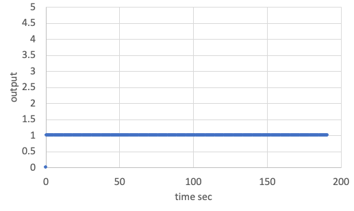
Result of constant offset noise (bias_noise_c = 1.0). -
Case 2:
normal_random_standard_deviation_c= 1.0, others = default- The simulation time is 1000sec, and the log output period is 0.1sec.
- The bottom figure shows the result of the output data.
- The calculated average and standard deviation from the output data are shown as follows.
Average = 0.012Standard Deviation = 1.000
- We verified the normal random noise calculation is correct according to the data.
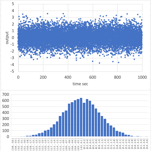
Result of normal random noise (normal_random_standard_deviation_c = 1.0). -
Case 3:
random_walk_standard_deviation_c= 0.3,random_walk_limit_c= 0.05, others = default- The simulation time is 200sec, and the log output period is 0.5sec.
- The bottom figure shows the result of the output data.
- The output data randomly varies inside the limit value.
- Note: The limit is not hard.
- We verified the normal random noise calculation is correct according to the data.
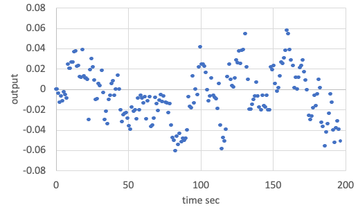
Result of Random Walk noise (random_walk_standard_deviation_c = 0.3, random_walk_limit_c = 0.05).
4. References
- N/A
Specification for StarSensor class
1. Overview
1. functions
StarSensorclass simulates a star sensor.- The
StarSensorclass calculates and returns the observed quaternions and error flags.
2. files
star_sensor.cpp, star_sensor.hpp: Definitions and declarations of the classstar_sensor.ini: Initialization fileplot_star_sensor.py: An example of a Python script to plot star sensor output
3. how to use
- Set the parameters in
star_sensor.ini. - Create an instance by using the initialization function
InitStarSensor - Use
Get*function to get quaternion information.
2. Explanation of Algorithm
1. Update
- TBW
2. Judgement
1. EarthJudgement
- Calculate the angle $\theta_{ce}$ between the earth's center direction $\boldsymbol{r_{sc}}$ and the earth's edge direction $\boldsymbol{r_{se}}$. $R_e$ is the earth's radius.
- Calculate the angle $\theta_{es}$ between the sight direction $\boldsymbol{r_{sight}}$ and the earth's edge direction $\boldsymbol{r_{se}}$.
- Judge the STT error flag by comparing $\theta_{es}$ with the earth forbidden angle $\theta_{efa}$. If $\theta_{es} > \theta_{efa}$, the earth is completely outside the earth forbidden angle.
\[ \begin{align} \theta_{ce} = \arctan{\left(\frac{|\boldsymbol{r_{se}}|}{R_e}\right)}\\ \theta_{cs} = \arccos{(\boldsymbol{r_{se}}*\boldsymbol{r_{sight}})}\\ \theta_{es} = \theta_{ce} - \theta_{cs} \tag{1} \end{align} \]
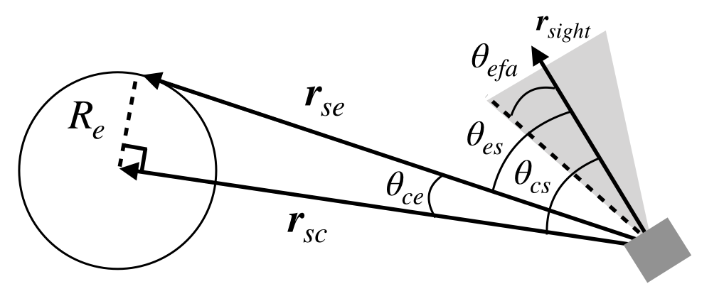
3. Results of verifications
1. verification of Earth judgement
1. overview
- Check that Earth judgement is performed correctly
2. conditions for the verification
- PropStepSec: 0.001
- StepTimeSec: 0.1
- EndTimeSec: 200
- Initial position [m] : [4.2164140100E+07,0,0]
- Initial velocity [m/s] : [0,3.074661E+03,0]
- ControlledAttitude
- main mode = EARTH_CENTER_POINTING: the pointing direction is determined by each case
- sub mode = SUN_POINTING: [0,0,1]
- STT quaternion from body frame to component frame: [0,0,0,1]
- Earth forbidden half-angle: 10deg
- The angle between the earth's center and edge direction: 8.6deg
3. results
- The angle between pointing direction and earth center = 15deg
- STT flag is always 1, since the angle $\theta_{es}$ between the sight direction and the earth's edge direction is 15 - 8.6 = 6.4deg < 10deg.
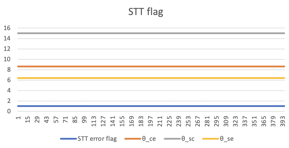
- The angle between pointing direction and earth center = 20deg
- STT flag is always 0, since the angle $\theta_{es}$ between the sight direction and the earth's edge direction is 20 - 8.6 = 11.4deg > 10deg.
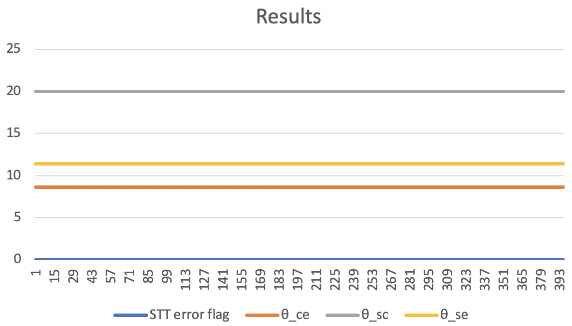
- The angle between pointing direction and earth center = 30deg
- STT flag is always 0, since the angle $\theta_{es}$ between the sight direction and the earth's edge direction is 30 - 8.6 = 21.4deg > 10deg.
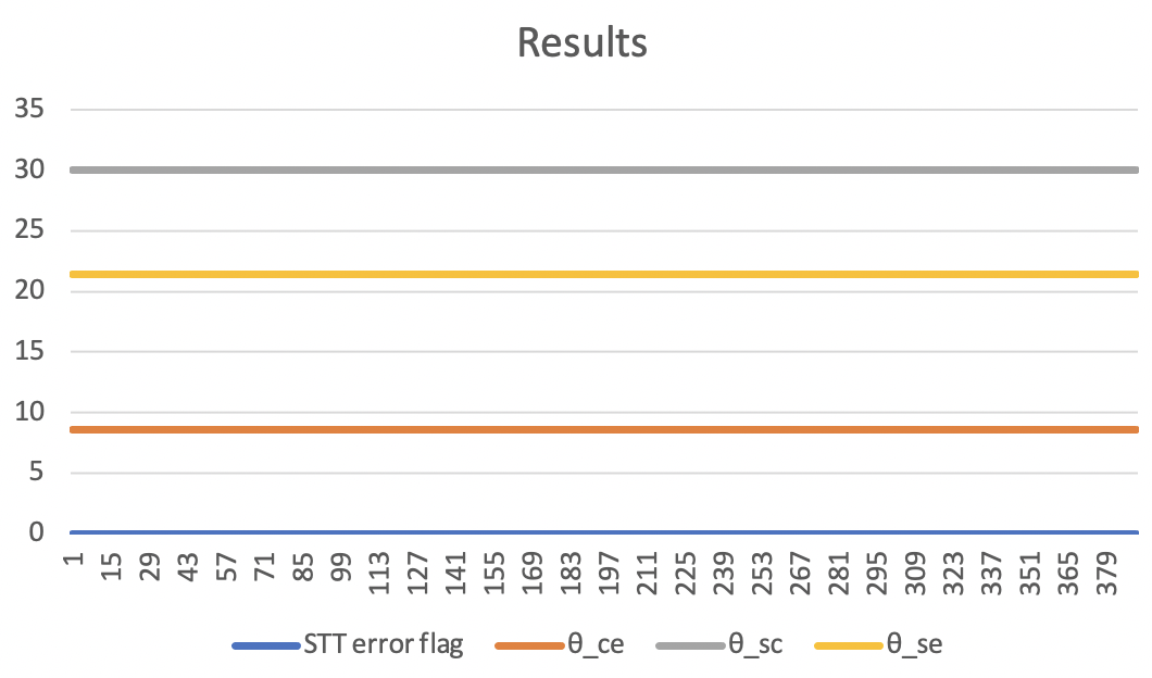
- The output result obtained by the default initial settings.
- The figure is generated by the Python script.
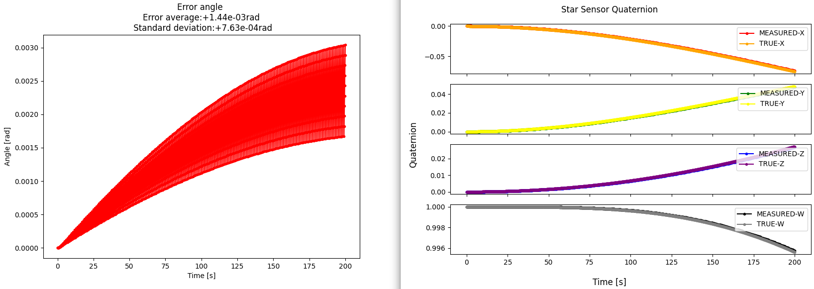
Specification for ReactionWheelJitter class
1. Overview
ReactionWheelJitterclass simulates the high-frequency jitter of Reaction Wheels.- This class uses:
- Angular velocity of the RW
- Parameters of RW disturbance measured by experiments
- This class returns:
- RW jitter forces and torques in the component frame
- RW jitter forces and torques in the body frame
1. functions
CalcJitter- Simulates the reaction wheel jitter
- (If Enabled) Calls
AddStructuralResonance(). This function adds the effect of structural resonance to the high-frequency disturbance of RW. You can choose to consider the effect of structural resonance or not.
2. files
reaction_wheel_jitter.cpp,reaction_wheel_jitter.hppreaction_wheel.iniradial_force_harmonics_coefficients.csv,radial_torque_harmonics_coefficients.csv- These files contain the harmonic coefficients from experiments.
3. how to use
- Set the harmonics coefficients in
radial_force_harmonics_coefficients.csvandradial_torque_harmonics_coefficients.csv - The first column is an array of the $h_i$( $i$-th harmonic number). The second column is an array of the $C_i$ (amplitude of the $i$-th harmonic).
- Set parameters in
reaction_wheel.ini - When only the static imbalance and dynamic imbalance(correspond to $C_i$ at $h_i\ne1$) is known according to the spec sheet, edit the files as follows.
radial_force_harmonics_coefficients.csv- Set $h_1$(the line 1 of the first column) as $1.0$.
- Set $C_1$(the line 1 of the second column) as the static imbalance on the spec sheet.
radial_torque_harmonics_coefficients.csv- Set $h_1$(the line 1 of the first column) as $1.0$.
- Set $C_1$(the line 1 of the second column) as the dynamic imbalance on the spec sheet.
reaction_wheel.ini- Set
harmonics_degree = 1.
- Set
- Set the jitter update period to an appropriate value.
- Jitter update period is equal to the product of
CompoUpdateIntervalSecinsimulation_base.iniandfast_prescalerinreaction_wheel.ini. - For correct calculation, the update period of the jitter should be set to approximately 0.1ms.
- A larger update period is not a problem, but it will cause aliasing in the jitter waveform.
- Jitter update period is equal to the product of
2. Explanation of Algorithm
1. CalcJitter
1. overview
- Function to calculate jitter force and torque
2. input and output
- input
- angular velocity of the RW
- output
- jitter force and torque in the component frame
- jitter force and torque in the body frame
3. algorithm
- The disturbances consist of discrete harmonics of reaction wheel speed with amplitudes proportional to the square of the wheel speed:
\[ u(t)=\sum_{i=1}^n C_i\Omega^2\sin(2\pi h_i\Omega t+\alpha_i) \]
- where $u(t)$ is the disturbance force and torque in Newton (N) or Newton-meters (Nm), $n$ is the number of harmonics included in the model, $C_i$ is the amplitude of the $i$ th harmonic in $\mathrm{N^2/Hz}$ (or $\mathrm{(Nm)^2/Hz}$), $\Omega$ is the wheel speed in Hz, $h_i$ is the $i$ th harmonic number and $\alpha_i$ is a random phase (assumed to be uniform over $[0, 2\pi]$) [1].
- $\alpha_i$ is generated as a uniform random number in the constructor.
- When users want to use a more precise model, set
considers_structural_resonanceto ENABLE inRW.iniand use a model that takes structural resonance inside the RW into account.- If structural resonances are not taken into account, the RW disturbance will be underestimated, but it is not a significant change in general.
- See the description of
AddStructuralResonance()for the algorithm to calculate the structural resonance.
2. AddStructuralResonance()
1. overview
- Function to add structural resonance inside the RW on the disturbance by harmonics of RW
2. input and output
- input:
- N/A
- output:
- jitter force and torque with structural resonance in component frame
3. algorithm
- The transfer function from disturbance by harmonics of RW without resonance ( $u(t)$ ) to disturbance with resonance ( $y(t)$ ) is modeled as following equation: \[ G(s)=\frac{s^2+2\zeta\omega_ns+\omega_n^2}{s^2+2d\zeta\omega_ns+\omega_n^2} \] \[ Y(s)=G(s)U(s) \]
- where $\omega_n$ is the angular frequency on the structural resonance. Other parameters such as $\zeta$, $d$ are determined by the result of experiments.
- To perform the simulation in discrete time, A bi-linear transformation $G(s)\rightarrow H(z)$ is applied. $T$ is the jitter update period.
\[ \begin{aligned} G(\frac{2}{T}\frac{z-1}{z+1})&=\dfrac{(\frac{2}{T}\frac{z-1}{z+1})^2+2\zeta\omega_n(\frac{2}{T}\frac{z-1}{z+1})+\omega_n^2}{(\frac{2}{T}\frac{z-1}{z+1})^2+2d\zeta\omega_n(\frac{2}{T}\frac{z-1}{z+1})+\omega_n^2}\\ &=\dfrac{(4+4\zeta T\omega_n+T^2\omega_n^2)+(-8+2T^2\omega_n^2)z^{-1}+(4-4\zeta T\omega_n+T^2\omega_n^2)z^{-2}}{(4+4d\zeta T\omega_n+T^2\omega_n^2)+(-8+2T^2\omega_n^2)z^{-1}+(4-4d\zeta T\omega_n+T^2\omega_n^2)z^{-2}}\\ &=\dfrac{c_3+c_4z^{-1}+c_5z^{-2}}{c_0+c_1z^{-1}+c_2z^{-2}}\\ &=H(z) \end{aligned} \]
- The $\omega_n$ should be the fixed value by pre-warping because there is frequency distortion due to bilinear transformation. The formula for calculating $\omega_n$ for the true resonant frequency $\omega_d$ is as follows:
\[ \omega_n=\frac{2}{T}\tan(\frac{T\omega_d}{2}) \]
- The bi-linear transformation transforms the relationship between input $u$ and output $y$ as follows:
\[ \begin{aligned} Y(z)&=H(z)U(z)\\ (c_0+c_1z^{-1}+c_2z^{-2})Y(z)&=(c_3+c_4z^{-1}+c_5z^{-2})U(z) \end{aligned} \]
-
By applying the inverse z-transform, the continuous relationship between $y(t)$ and $u(t)$ can be expressed as a discrete relationship of a difference equation between $y[n]$ and $u[n]$, where $[n]$ is the current simulation time step. The difference equation is as follows: \[ c_0y[n]+c_1y[n-1]+c_2y[n-2]=c_3u[n]+c_4u[n-1]+c_5u[n-2] \]
-
Therefore, $y[n]$ is calculated as follows. \[ y[n]=\frac{(-c_1y[n-1]-c_2y[n-2]+c_3u[n]+c_4u[n-1]+c_5u[n-2])}{c_0} \]
3. Results of verifications
- In this section, jitter output when the RW is rotated at a constant speed is verified.
1. X-axis torque data in the time domain
1. overview
- The RW model is rotated at 4000 rpm, 6000 rpm, and 8000 rpm, and the disturbance torque is compared with the actual experiment.
2. initial condition
- input files
sample_simulation_base.inireaction_wheel.ini
- initial condition
sample_simulation_base.iniEndTimeSec = 0.5 StepTimeSec = 0.0001 CompoUpdateIntervalSec = 0.0001 LogOutputIntervalSec = 0.0001reaction_wheel.inifast_prescaler = 1 max_angular_velocity = 9000.0 calculation = ENABLE logging = ENABLE harmonics_degree = 12 considers_structural_resonance = ENABLE structural_resonance_freq = 585.0 //[Hz] damping_factor = 0.1 //[ ] bandwidth = 0.001 //[ ]
3. result
- The simulation result is compared with the disturbance experiment result of Sinclair RW0.003.
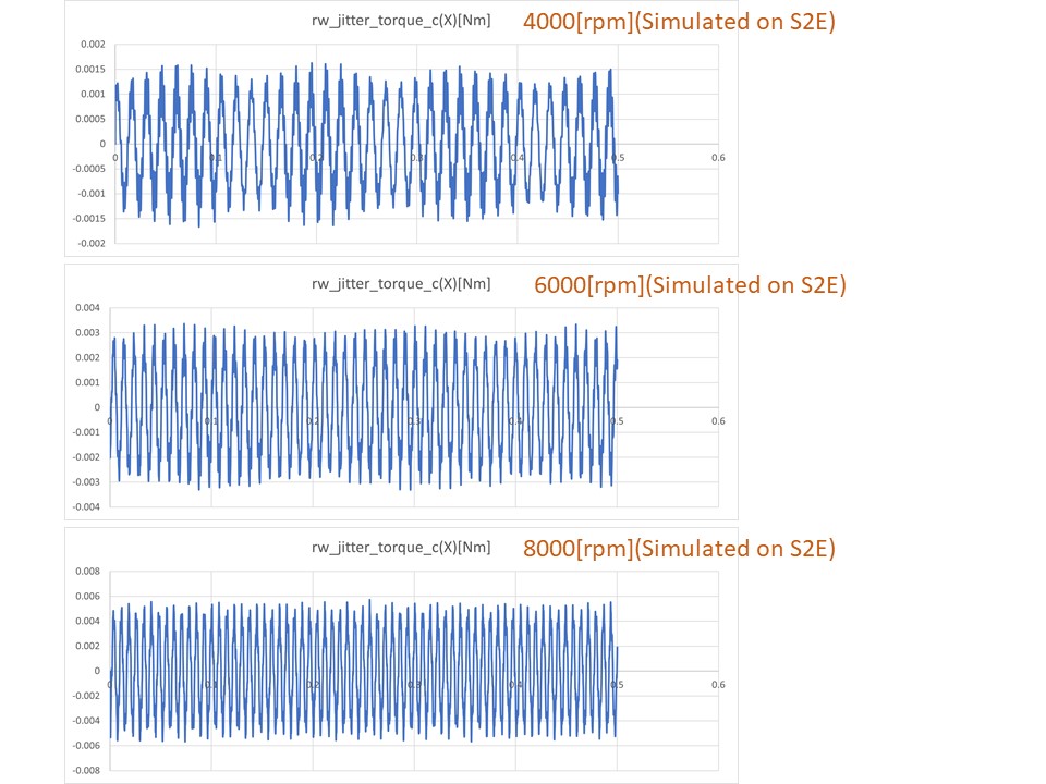
- At all speeds, the characteristics of the actual RW are well simulated.
2. X-axis torque waterfall
1. overview
- The RW model is rotated at 1000, 2000, ..., 9000rpm, and the jitter torque time-domain data was extracted. Then, FFT was applied to the data by Matlab, and the waterfall plot was plotted.
2. initial condition
- same as the initial condition of the verification about the time domain data
3. result
- The simulation result is compared with the disturbance experiment result of Sinclair RW0.003.
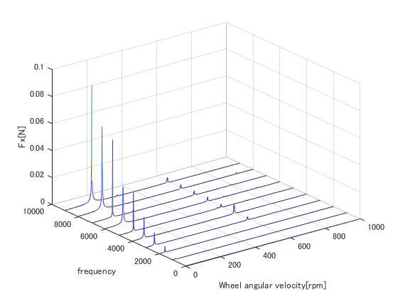
- Both the first-order mode and the structural resonance ($\omega_n=585\mathrm{Hz}$) are approximately simulated.
4. References
- Masterson, R. A. (1999). Development and validation of empirical and analytical reaction wheel disturbance models (Doctoral dissertation, Massachusetts Institute of Technology).
- Shields, et al., (2017). Characterization of CubeSat reaction wheel assemblies. Journal of Small Satellites, 6(1), 565-580.
Specification for Telescope
1. Overview
- This class simulates a telescope.
- This class uses the position information of celestial bodies and returns the following data:
- Flags that show whether the bright celestial bodies(the Earth, the Moon, and the Sun) are in the forbidden angle of the telescope
- Positions of the celestial bodies on the image sensor
- Positions of stars on the image sensor
1. functions
MainRoutineruns the following three functions:JudgeForbiddenAngle- Function to judge whether the celestial body is in the forbidden angle.
Observe- Function to
- judge whether the celestial body(provided by
CelesInfo) is in the field of view. - output position of its image on the image sensor, if it is in the field of view.
- judge whether the celestial body(provided by
- Function to
ObserveStars- Function to output some HIP IDs of the brightest stars in the field of view, using
HipparcosCatalogue. - Specify how many stars this function outputs in
telescope.ini.
- Function to output some HIP IDs of the brightest stars in the field of view, using
2. files
telescope.cpp,telescope.hpp- Definitions and declarations of the class
hipparcos_catalogue.cpp,hipparcos_catalogue.hpp- Definitions and declarations of the class to read Hipparcos catalogue.
3. how to use
- Set the parameters in
telescope.ini - Create instance by using initialization function
InitTelescope.- Each telescope is numbered as "Telescope1,…"
- To use
HipparcosCataloguedata,hip_main.csvis necessary.s2e-core/scripts/Common/download_HIPcatalogue.shis the script to download it. Run the following code using Git bash ins2e-core/scripts/:bash download_HIPcatalogue.sh
2. Explanation of Algorithm
1. JudgeForbiddenAngle
1. overview
- Function to judge whether a celestial body is in the forbidden angle.
2. input and output
- input
- The position vector of the celestial body in the body-fixed coordinate.
- This position vector is provided by
CelestialInformation.
- This position vector is provided by
- The forbidden angle about the celestial body
- Specify the forbidden angle in
telescope.ini.
- Specify the forbidden angle in
- The position vector of the celestial body in the body-fixed coordinate.
- output
- true: The celestial body is in forbidden angle
- false: The celestial body is not in forbidden angle
3. process to judge
- The judging process is calculated in the telescope's component coordinate. $q_{b2c}$ is the quaternion to convert from the body coordinate(B) to the component coordinate(C). Specify $q_{b2c}$ in
telescope.ini. The X-axis of the component coordinate is defined as the line of sight of the telescope.
2. Observe
1. overview
- This function judges whether the celestial bodies(provided by
CelestialInformation) are in the field of view and outputs the position of them on the image sensor if they are in the field of view - If they are not in the field of view, this function outputs $(-1,-1)$.
2. input and output
- input
- The reference to the position of the celestial body on the image sensor
- The position vector of the celestial body in the body-fixed coordinate
CelestialInformationprovides the position vector.
- output
- (void)
- This function rewrites the "reference to the celestial body's position on the image sensor" given as the input.
- (void)
3. algorithm
1. Calculate process to judge whether the celestial body is in the field of view
- A 2D coordinate on the image sensor is defined to handle the position on the image sensor. The definition is as follows:
- The X-axis of the image sensor coordinate corresponds with the Z-axis of the component coordinate.
- The Y-axis of the image sensor coordinate corresponds with the Y-axis of the component coordinate.
- Then, the inclination angle from the X-axis of the celestial body's direction in the XZ plane of the component coordinate is calculated using $(x_c, y_c, z_c)$ as follows:
\[ tan^{-1}\frac{z_c}{x_c} \]
- In the same way, the inclination angle from the X-axis of the celestial body's direction in the XY plane of the component coordinate is calculated as follows:
\[ tan^{-1}\frac{y_c}{x_c} \]
- They are written as
arg_xandarg_yin the code. In this manual, $\theta_x$ and $\theta_y$ are used for them. If $\theta_x$ is within FOV_x and $\theta_y$ is within FOV_y, the celestial body is judged to be in the field of view.
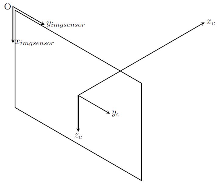
2. Calculate process for calculating the position of the image
- The origin of the sensor coordinate is the corner of the image sensor, so $x_{imgsensor}$ and $y_{imgsensor}$ have positive values. The unit of them is pixel(pix). In this manual, $N_x$ and $N_y$ are used for the total number of pixels along x, y axes of the sensor coordinate (They are
x_num_of_pixandy_num_of_pixin the code). In the same way,XandYare used for the position of the celestial body on the image sensor (They arepos_imgsensor[0]andpos_imgsensor[1]). Then,XandYare calculated as follows: \[ X=\frac{N_x}{2}\times\frac{\tan(\theta_x)}{\tan(FOV_x)}+\frac{N_x}{2} \] \[ Y=\frac{N_y}{2}\times\frac{\tan(\theta_y)}{\tan(FOV_y)}+\frac{N_y}{2} \]
If the celestial body is not in the field of view, the output is $X=Y=-1$.
3. ObserveStars
1. overview
- Function to output some HIP IDs of the brightest stars in the field of view, using
HipparcosCatalogue
2. input and output
- input
- (void)
- output
- (void)
3. main process
When ObserveStars is called in the MainRoutine, this function works as follows:
- Clear
star_in_sight - Judge the brightest star (provided by
HipparcosCatalogue) is in the field of view - If the star is in the field of view, push the information (such as the HIP ID and its position on the image sensor) to
star_in_sight - Go to step 2. to judge the next brightest star
- Exit the loop when the number of elements of
star_in_sightreaches the specified number
4. error handling
If all the data in HipparcosCatalogue are checked before the number of elements of star_in_sight reaches the specified number, the data of lacking element is filled with -1.
3. Results of verifications
In this section, the output of the functions when some angular velocity is input is verified.
1. Input of angular velocity around X-axis of the body coordinate
1. overview
- input $ω_b=[0.1~0~0]^T$ .
2. conditions for the verification
- input files
sample_simulation_base.initelescope.ini
- initial condition
sample_simulation_base.iniSimulation start date[UTC] : 2017/12/01 11:00:00.0 Simulation finish time[sec] : 1500 Quaternion : q_i2b=[0 0 0 1]^Ttelescope.iniq_b2c=[0 0 0 1]^T sun_forbidden_angle = 60 earth_forbidden_angle = 60 moon_forbidden_angle = 60 x_num_of_pix = 2048 y_num_of_pix = 2048 x_fov_par_pix = 0.02 y_fov_par_pix = 0.02sample_simulation_base.ini[HIPPARCOS_CATALOGUE] max_magnitude = 5.0 calculation = ENABLE logging = DISABLE
The disturbance torque in the main function of sample_case.cpp is commented out.
3. result
- judge for forbidden angle
- The angle from the line of sight about the direction of the Sun, the Earth, the Moon is as follows:
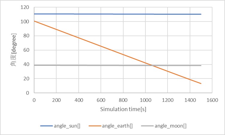
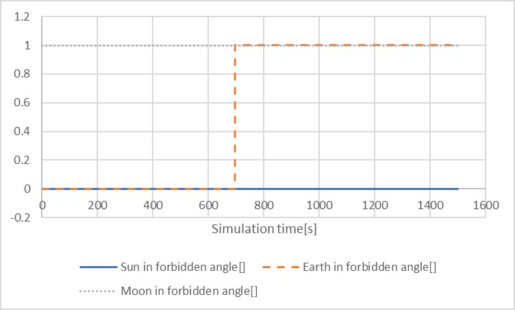
Observefunction- Only the Moon and the Earth are in the field of view (See the figure "The angle from the line of sight about the direction of the Sun, the Earth, the Moon"). The track of the image of the Moon on the image sensor is as follows:
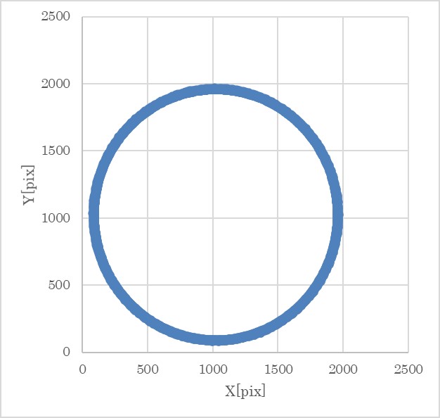
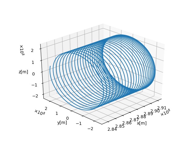
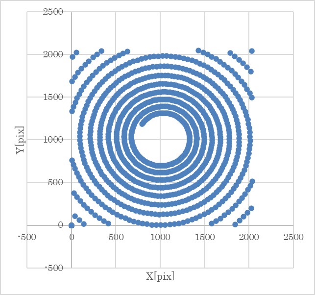
In addition, the 3D plot of EARTH_POS_B is as follows:
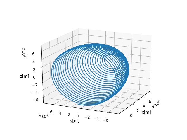
ObserveStarsfunction
- The first, second, and third HIP ID outputs were 113368, 9884, and 3419. Their track on the image sensor are as follows:
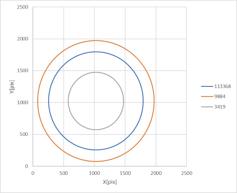
The tracks make circles, which are the reasonable outputs because of the same reason stated in the verification of Observe function. In addition, the each Vmag of HIP ID=113368,9884,and 3419 is 1.17,2.01,and 2.04, so it is verified that the outputs are in order of brightness.
2. input of angular velocity around y axis of the body coordinate
1. overview
- The angular velocity input is $ω_b=[0.1~0~0]^T$ .The other condition is the same as the case of 1. Note that the verification of the case around z axis is omitted because y and z are equivalent under this condition.
2. result
- judge for forbidden angle
- The angle from the line of sight about the direction of the Sun, the Earth, the Moon is as follows:
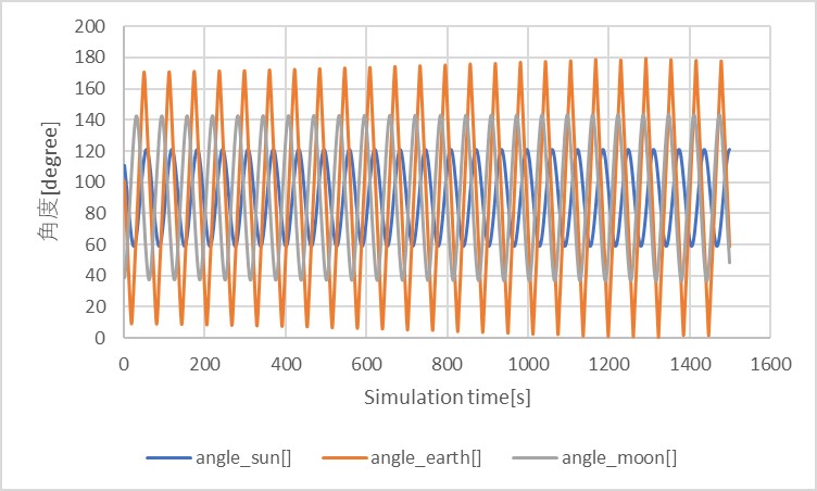
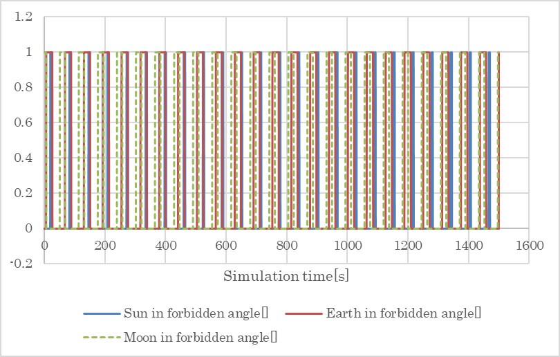
Observefunction
- The figure "The angle from the line of sight about the direction of the Sun, the Earth, the Moon" shows that the earth is mainly in the field of view, so this section discusses only about the Earth. The track of the image of the Earth is as follows (For the sake of ease, only 4 tracks in the field of view are displayed):
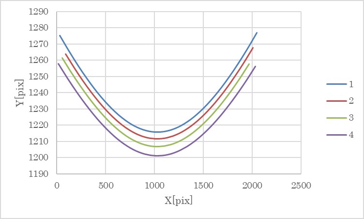
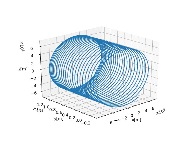
ObserveStarsfunction
- The tracks of the stars are partially as follows:
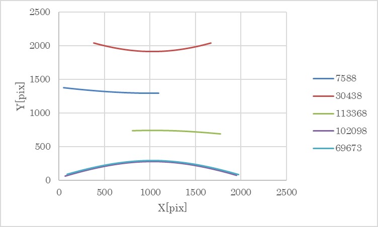
4. References
Specification of PowerControlUnit class
1. Overview
1. Functions
PowerControlUnitclass is a base class of power control units and manages multiplePowerPorts.
2. Related files
- Main file:
power_control_unit.cpp, .hpp - Related file:
power_port.cpp, .hpp
3. How to use
- Example: The
sample_componentsin thes2e-core/simulation_sample/spacecraftis useful to know how to use this class. - Users can make their original
PowerControlUnitclass by inheriting this base class. - Users need to override the
MainRoutine,GetLogHeader, andGetLogValuefunctions to define the behavior of their PCUs.
2. Explanation of Algorithm
1. ConnectPort
1. overview
- This function makes a new
PowerPort.
2. inputs and outputs
- Inputs: the port ID and the arguments for
PowerPort - Outputs: the error code (0 is a success, -1 is an error)
3. algorithm
- Make a new
PowerPortwhen the port ID is not used.
4. note: N/A
2. ClosePort
1. overview
- This function deletes the designated
PowerPort.
2. inputs and outputs
- Inputs: the port ID.
- Outputs: the error code (0 is a success, -1 is an error).
3. algorithm
- Delete the designated
PowerPortwhen the port still exists.
4. note: N/A
3. Results of verifications
N/A
4. References
N/A
Specification for Thruster
1. Overview
- This class simulates a thruster and contains functions for it.
1. functions
- By setting the thruster valve open and close, thruster torque and force are generated.
- The thruster model includes the magnitude and directional errors in the ini file.
- According to the thruster output, users can set the thrust duty to the value between 0 and 1.
2. files
simple_thruster.cpp,simple_thruster.hpp- Definitions and declarations of the class
thruster.ini- Parameters for a/multiple thruster(s)
plot_simple_thruster.py: An example of a Python script to plot simple thruster output
3. how to use
- Set the parameters written in
thruster.ini.- Users can set multiple thrusters.
- Create an instance by
SimpleThrusterfunction. - Add
calc_thrustfunction toGenerateForce_b()inSatComponentsclass andcalc_torquefunction toGenerateTorque_b()inSatComponentsclasscalc_torquefunction requires a position of the spacecraft's mass center as an argument.
- When a thruster is open, set the duty to 1 by
set_duty(1)function.- Users can set duty to the value between 0 and 1.
2. Explanation of Algorithm
1. Thrust
1. overview
- Thrust magnitude is a scalar value of thrust.
- Thrust contains the magnitude and direction errors according to the ini file setting.
- Thrust magnitude calculation considers the duty of thruster. If the thruster valve is closed, the thrust magnitude is 0.
2. input and output
- input
- Thruster duty ratio
- Maximum thrust magnitude
thrust_magnitude_N - Thrust direction
thruster_direction_b - Thrust magnitude error
thrust_error_standard_deviation_N - Thrust direction error
direction_error_standard_deviation_deg
- output
- Thrust magnitude and direction
3. algorithms
Thrust magnitude can be calculated as follows:
\[ F_{thrust} = \epsilon * F_{max} + n_{f} \]
where $F_{thrust}$ is thrust magnitude, $\epsilon$ is the duty of thruster, $F_{max}$ is the maximum thrust magnitude, and $n_{f}$ is the error of thrust magnitude.
Thrust direction can be calculated as follows:
\[ \boldsymbol{d}_{err} = \boldsymbol{q}(\boldsymbol{d}_{true},n) * \boldsymbol{d}x \] \[ \boldsymbol{d}_{thrust} = \boldsymbol{q}(\boldsymbol{d}_{err},n{d}) * \boldsymbol{d}_{true} \]
where
- $\boldsymbol{d}_{true}$ is the thrust vector without errors
- $n$ is the random angles to rotate the direction of error $\boldsymbol{d}_{err}$
- $\boldsymbol{d}_{x}$ is the vector which is not equal to $\boldsymbol{d}_{true}$
- $n_d$ is the directional error
- $\boldsymbol{d}_{thrust}$ is the thrust vector with errors
- $\boldsymbol{q}(\boldsymbol{d},n)$ is the quaternion which has the rotation axis $\boldsymbol{d}$ and the rotation angle $n$ .
Thrust can be calculated as follows:
\[ \boldsymbol{F}_{thrust} = F_{thrust} * \boldsymbol{d}_{thrust} \]
where $\boldsymbol{F}_{thrust}$ is thrust.
2. Torque
1. overview
- Torque by thruster is calculated from the thrust vector and the vector between the center of mass of the spacecraft and thruster.
2. input and output
- input
- Thruster position
thruster_position_b_m - Mass center of spacecraft
- Thrust magnitude and direction
- Thruster position
- output
- Torque
3. algorithms
Torque by the thruster can be calculated as follows:
\[ \boldsymbol{T}_{thrust} = (\boldsymbol{v}_{thruster}-\boldsymbol{v}_{SC}) \times \boldsymbol{F}_{thrust} \]
where
- $\boldsymbol{T}_{thrust}$ is torque by the thruster
- $\boldsymbol{v}_{thruster}$ is thruster position
- $\boldsymbol{v}_{SC}$ is the mass center of spacecraft.
3. Results of verifications
1. Case1
-
input
- Position
thruster_position_b_m: [0m, 0m, 0.1m] - Direction
thruster_direction_b: [0, 0, 1] - Thrust magnitude
thrust_magnitude_N: 0.001N - Thrust magnitude error
thrust_error_standard_deviation_N: 0.0N - Thrust direction error
direction_error_standard_deviation_deg: 0.0deg - Simulation time: 100sec
- Position
-
result
-
Force Mean: [0,0,0.001] N
-
Force Std Dev: [0,0,0] N
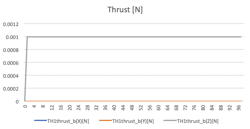
Thrust force values in N unit. -
Torque Mean: [0,0,0] Nm
-
Torque Std Dev: [0,0,0] Nm
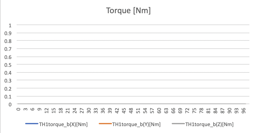
Thrust torque values in Nm unit.
-
2. Case2
- input
- Position
thruster_position_b_m: [0, 0, 0.1] m - Direction
thruster_direction_b: [0, 0, 1] - Thrust magnitude
thrust_magnitude_N: 0.001N - Thrust magnitude error
thrust_error_standard_deviation_N: 0.00001N - Thrust direction error
direction_error_standard_deviation_deg: 0.0deg - Simulation time: 100sec
- Position
- result
-
Force Mean: [0,0,0.999611e-3] N
-
Force Std Dev: [0,0,1.09804e-5] N
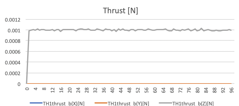
Thrust force values in N unit. -
Torque Mean: [0,0,0] Nm
-
Torque Std Dev: [0,0,0] Nm
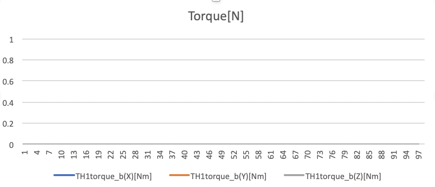
Thrust torque values in Nm unit.
-
3. Case3
- input
- Position
thruster_position_b_m: [0, 0, 0.1] m - Direction
thruster_direction_b: [0, 0, 1] - Thrust magnitude
thrust_magnitude_N: 0.001N - Thrust magnitude error
thrust_error_standard_deviation_N: 0.0N - Thrust direction error
direction_error_standard_deviation_deg: 10.0deg - Simulation time: 100sec
- Position
- result
-
Force Mean: [-4.93e-6, -1.04e-5, 0.9834e-3] N
-
Force Std Dev: [1.0e-4, 9.79e-5, 1.216e-5] N
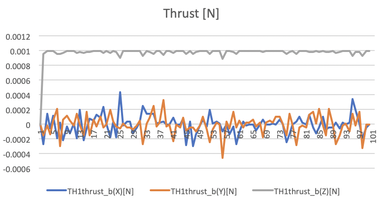
Thrust force values in N unit. -
Torque Mean: [1.04e-6,-4.94e-7,0] Nm
-
Torque Std Dev: [1.29e-5, 1.26e-5, 0] Nm
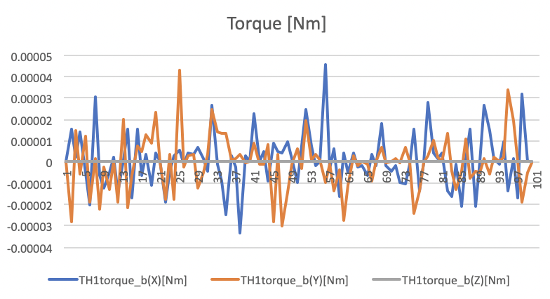
Thrust torque values in Nm unit.
-
4. Case4
- input
- Position
thruster_position_b_m: [0, 0.1, 0] m - Direction
thruster_direction_b: [0, 0, 1] - Thrust magnitude
thrust_magnitude_N: 0.001N - Thrust magnitude error
thrust_error_standard_deviation_N: 0.0N - Thrust direction error
direction_error_standard_deviation_deg: 0.0deg - Simulation time: 100sec
- Position
- result
-
Force Mean: [0,0,0.001] N
-
Force Std Dev: [0,0,0] N
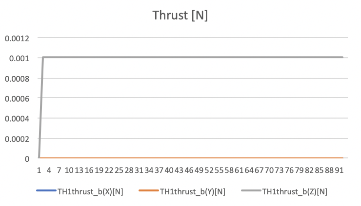
Thrust force values in N unit. -
Torque Mean: [0.0001,0,0] Nm
-
Torque Std Dev: [0,0,0] Nm
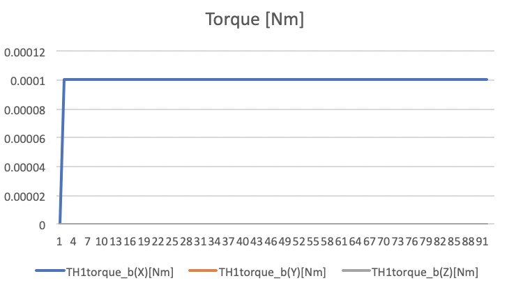
Thrust torque values in Nm unit.
-
Specification of Geopotential Calculation
1. Overview
1. Functions
- The
Geopotentialclass calculates the gravity acceleration of the earth with the EGM96 geo-potential model.
2. Related files
src/disturbances/geopotential.cpp, .hppsrc/library/gravity/gravity_potential.cpp, .hpps2e-core/ExtLibraries/GeoPotential/egm96_to360.ascii- The EGM96 geopotential coefficients file was downloaded from NASA's EMG96 website, but we cannot access it now.
3. How to use
- Make an instance of the
Geopotentialclass inInitializeInstancesfunction indisturbances.cpp- Create an instance by using the initialization function
InitGeopotential
- Create an instance by using the initialization function
- Choose an orbit propagator mode that considers disturbances.
- Edit the
disturbance.inifile- Select
ENABLEforcalculationandlogging - Select
degreeof calculation- When the
degreeis smaller than 1, it is overwritten as 0. - When the
degreeis larger than 360, it is overwritten as 360. - NOTE: The calculation time is related to the selected degree.
- When the
- Select
2. Explanation of Algorithm
- The base algorithm is referred to Satellite Orbits chapter 3.2.
1. Read coefficients
1. overview
- This function reads the geopotential coefficients from the EGM96 file
egm96_to360.ascii. - The file doesn't have coefficients for
n=0,m=0,n=1,m=0, andn=1,m=1. - All coefficients are completely normalized by following normalization function $N_{n,m}$
\[ N_{n,m}=\sqrt{\frac{(n+m)!}{(2-\delta_{0m})(2n+1)(n-m)!}}\\ \]
- where $\delta_{0m}$ is the Kronecker delta.
2. inputs and outputs
- Input
- file path of
egm96_to360.ascii - maximum degree for geopotential calculation
- file path of
- Output
- Return: reading is succeeded or not.
- Normalized coefficient $C_{n,m}$ and $S_{n,m}$
- algorithm
- The file format of
egm96_to360.asciiisn,m,Cnm,Snm,sigmaCnm,sigmaSnmin line with space delimiter. In this calculation, thesigmaCnmandsigmaSnmare not used. - The total number of reading lines is defined as the following equation
\[
N_{line}=\frac{1}{2}(n+1)(n+2)-3
\]
- where $n$ is maximum degree, and -3 is for the coefficients of
n=0,m=0,n=1,m=0, andn=1,m=1, which are not in the file.
- where $n$ is maximum degree, and -3 is for the coefficients of
- note
- When the reading file process is failed, the maximum degree is set to zero, and a simple Kepler calculation will be executed.
2. Calculate Legendre polynomials with recursion algorithm
1. overview
- We chose to use the recursion algorithm written in chapter 3.2.4 of Satellite Orbits since the calculation of the Legendre polynomials for spherical harmonics is time-consuming.
- However, the original equation in the book is unnormalized form, and it is not suitable with the normalized coefficients.
- For a small degree, users can directly use the normalized function $N_{n,m}$ to unnormalize the coefficients or to normalize the functions $V_{n,m}$ and $V_{n,m}$ . But for a large degree, the factorial calculation in the $N_{n,m}$ reaches a huge value, which standard
doublevariables cannot handle. - To avoid that, the normalized recursion algorithm was derived as described in Section 3.
- There are the following two functions:
v_w_nn_updatev_w_nm_update
2. inputs and outputs
- Inputs
- Both functions
- Satellite position in ECEF frame $x, y, z$
- degree and order as $n$ and $m$
v_w_nn_update: $V_{n-1,n-1}$ and $W_{n-1,n-1}$v_w_nm_update: $V_{n-1,m}, W_{n-1,m}, V_{n-2,m}$, and $W_{n-2,m}$
- Both functions
- Outputs
v_w_nn_update: $V_{n,n}$ and $W_{n,n}$v_w_nm_update: $V_{n,m}$ and $W_{n,m}$
3. algorithm
For unnormalized algorithms, see chapter 3.2.4 of Satellite Orbits.
For normalized algorithm, we use following normalizing relation for Legendre polynomials,
\[ \begin{align} \bar{P}_{n,m} &= \frac{1}{N_{n,m}}P_{n,m}\\ \bar{V}_{n,m} &= \frac{1}{N_{n,m}}V_{n,m}\\ \bar{W}_{n,m} &= \frac{1}{N_{n,m}}W_{n,m}\\ \end{align} \]
The recursion calculation of V and W can be changed to a normalized version as follows
\[ \begin{align} N_{m,m}\bar{V}_{m,m} &= (2m-1)(\frac{xR_{e}}{r^2}N_{m-1,m-1}\bar{V}_{m-1,m-1}-\frac{yR_e}{r^2}N_{m-1,m-1}\bar{W}_{m-1,m-1})\\ \bar{V}_{m,m} &= \frac{N_{m-1,m-1}}{N_{m,m}}(2m-1)(\frac{xR_{e}}{r^2}\bar{V}_{m-1,m-1}-\frac{yR_e}{r^2}\bar{W}_{m-1,m-1})\\ \bar{W}_{m,m} &= \frac{N_{m-1,m-1}}{N_{m,m}}(2m-1)(\frac{xR_{e}}{r^2}\bar{W}_{m-1,m-1}+\frac{yR_e}{r^2}\bar{V}_{m-1,m-1})\\ \end{align} \]
\[ \begin{align} N_{n,m}\bar{V}_{n,m} &= \frac{2n-1}{n-m}(\frac{zR_{e}}{r^2}N_{n-1,m}\bar{V}_{n-1,m}-\frac{n+m-1}{n-m}\frac{R_e^2}{r^2}N_{n-2,m}\bar{V}_{n-2,m})\\ \bar{V}_{n,m} &= \frac{2n-1}{n-m}\frac{zR_{e}}{r^2}\frac{N_{n-1,m}}{N_{n,m}}\bar{V}_{n-1,m}-\frac{n+m-1}{n-m}\frac{R_e^2}{r^2}\frac{N_{n-2,m}}{N_{n,m}}\bar{V}_{n-2,m}\\ \bar{W}_{n,m} &= \frac{2n-1}{n-m}\frac{zR_{e}}{r^2}\frac{N_{n-1,m}}{N_{n,m}}\bar{W}_{n-1,m}-\frac{n+m-1}{n-m}\frac{R_e^2}{r^2}\frac{N_{n-2,m}}{N_{n,m}}\bar{W}_{n-2,m}\\ \end{align} \]
The recurrence relation of normalize function can be expressed as follows
\[ \begin{align} N_{0,0} &= 1\\ N_{m,m} &= (2m-1)\sqrt{\frac{2m}{2m+1}}N_{m-1,m-1}\quad(m\geq1)\\ N_{n,m} &= \sqrt{\frac{2n-1}{2n+1}}\sqrt{\frac{n+m}{n-m}}N_{n-1,m}\quad(n\geq1,0\leq m \leq n) \end{align} \]
So, the divisions of the normalized functions are described as follows \[ \begin{align} \frac{N_{0,0}}{N_{1,1}} &= \sqrt{2m+1}=\sqrt{3}\\ \frac{N_{m-1,m-1}}{N_{m,m}} &= \frac{1}{2m-1}\sqrt{\frac{2m+1}{2m}}\quad(m\geq2)\\ \frac{N_{n-1,m}}{N_{n,m}} &= \sqrt{\frac{2n+1}{2n-1}}\sqrt{\frac{n-m}{n+m}}\quad(n\geq1,0\leq m \leq n)\\ \frac{N_{n-2,m}}{N_{n,m}} &= \frac{N_{n-2,m}}{N_{n-1,m}}\frac{N_{n-1,m}}{N_{n,m}}\\ \frac{N_{n-2,m}}{N_{n,m}} &= \sqrt{\frac{2n-1}{2n-3}}\sqrt{\frac{n-m-1}{n+m-1}}\frac{N_{n-1,m}}{N_{n,m}}\quad(n\geq2,0\leq m \leq n) \end{align} \] The recurrence relations for normalized V and W are derived as follows \[ \begin{align} \bar{V}_{0,0} &= \frac{Re}{r}\\ \bar{W}_{0,0} &= 0\\ \bar{V}_{1,1} &= \sqrt{3}(2m-1)(\frac{xR_{e}}{r^2}\bar{V}_{0,0}-\frac{yR_e}{r^2}\bar{W}_{0,0})\\ \end{align} \] \[ \begin{align} \bar{V}_{m,m} &= \sqrt{\frac{2m+1}{2m}}(\frac{xR_{e}}{r^2}\bar{V}_{m-1,m-1}-\frac{yR_e}{r^2}\bar{W}_{m-1,m-1})\quad(m\geq2)\\ \bar{W}_{m,m} &= \sqrt{\frac{2m+1}{2m}}(\frac{xR_{e}}{r^2}\bar{W}_{m-1,m-1}+\frac{yR_e}{r^2}\bar{V}_{m-1,m-1})\quad(m\geq2)\\ \end{align} \] \[ \begin{align} \bar{V}_{n,m} &= \sqrt{\frac{2n+1}{2n-1}}\sqrt{\frac{n-m}{n+m}}(\frac{2n-1}{n-m}\frac{zR_{e}}{r^2}\bar{V}_{n-1,m})\quad(n=1,0\leq m \leq n)\\ \bar{W}_{n,m} &= \sqrt{\frac{2n+1}{2n-1}}\sqrt{\frac{n-m}{n+m}}(\frac{2n-1}{n-m}\frac{zR_{e}}{r^2}\bar{W}_{n-1,m})\quad(n=1,0\leq m \leq n)\\ \end{align} \] \[ \begin{align} \bar{V}_{n,m} &= \sqrt{\frac{2n+1}{2n-1}}\sqrt{\frac{n-m}{n+m}}(\frac{2n-1}{n-m}\frac{zR_{e}}{r^2}\bar{V}_{n-1,m}-\frac{n+m-1}{n-m}\frac{R_e^2}{r^2}\sqrt{\frac{2n-1}{2n-3}}\sqrt{\frac{n-m-1}{n+m-1}}\bar{V}_{n-2,m})\quad(n\geq2,0\leq m \leq n)\\ \bar{W}_{n,m} &= \sqrt{\frac{2n+1}{2n-1}}\sqrt{\frac{n-m}{n+m}}(\frac{2n-1}{n-m}\frac{zR_{e}}{r^2}\bar{W}_{n-1,m}-\frac{n+m-1}{n-m}\frac{R_e^2}{r^2}\sqrt{\frac{2n-1}{2n-3}}\sqrt{\frac{n-m-1}{n+m-1}}\bar{W}_{n-2,m})\quad(n\geq2,0\leq m \leq n)\\ \end{align} \]
3. Calculate acceleration: CalcAccelerationECEF
1. overview
- This function calculates gravity acceleration
2. inputs and outputs
- Input
- normalized coefficients
- $\bar{C}_{n,m}$
- $\bar{S}_{n,m}$
- normalized function
- $\bar{V}_{n,m}$
- $\bar{W}_{n,m}$
- normalized coefficients
- Output
- Gravity acceleration in ECEF frame
3. algorithm
For unnormalized algorithms, See chapter 3.2.5 of Satellite Orbits.
When we use the normalized coefficients and normalized functions, the acceleration calculation is described like follows \[ \begin{align} \ddot{x}_{n,m} &= -\frac{GM}{Re^{2}}\bar{C}_{n,0}\bar{V}_{n+1,1}\\ &= -\frac{GM}{Re^{2}} C_{n,0}V_{n+1,1} \frac{N_{n,0}}{N_{n+1,1}}\quad(m=0) \end{align} \] The division of normalized function $\frac{N_{n,0}}{N_{n+1,1}}$ should be removed, so we have to multiply following correction factors into the equation.
When $m=0$, following correction factors are useful for x and y acceleration \[ \begin{align} \frac{N_{n+1,1}}{N_{n,0}}=\sqrt{\frac{1}{2}}\sqrt{\frac{2n+1}{2n+3}}\sqrt{(n+2)(n+1)} \end{align} \] When $m=1$, following correction factors are useful for x and y acceleration \[ \begin{align} \frac{N_{n+1,0}}{N_{n,1}}=\sqrt{2}\sqrt{\frac{2n+1}{2n+3}}\sqrt{\frac{1}{n(n+1)}}\quad(m=1)\\ \end{align} \] When $m>1$, following correction factors are useful for x and y acceleration \[ \begin{align} \frac{N_{n+1,m+1}}{N_{n,m}} &= \sqrt{\frac{2n+1}{2n+3}}\sqrt{(n+m+1)(n+m+2)}\\ \frac{N_{n+1,m-1}}{N_{n,m}} &= \sqrt{\frac{2n+1}{2n+3}}\sqrt{\frac{1}{(n-m+1)(n-m+2)}}\\ \end{align} \] When $m>=0$, following correction factors are useful for z acceleration \[ \begin{align} \frac{N_{n+1,m}}{N_{n,m}}=\sqrt{\frac{2n+1}{2n+3}}\sqrt{\frac{n+m+1}{n-m+1}} \end{align} \]
4. note
- To accelerate the calculation, the double
for loopof acceleration calculation and the recursion loop need to be integrated in future.
3. Results of verifications
1. Calculation accuracy
1. overview
- The calculated gravity acceleration is compared with Matlab's Gravity Spherical Harmonics calculation.
- The satellite position in the ECEF frame calculated by S2E is inputted to the
CalcAccelerationECEFandgravitysphericalharmonic( r, 'EGM96',360, 'Error' );function of Matlab.- Both calculations use EGM96.
- The degree of Matlab is fixed to 360, the degree of S2E is changed to check the relationship between the degree and the accuracy.
2. conditions for the verification
-
input files
- Default initialize files
-
initial values
-
Default initialize files
simulation_start_time_utc = 2020/01/01 11:00:00.0 simulation_duration_s = 200 simulation_step_s = 0.1 orbit_update_period_s = 0.1 log_output_period_s = 5 simulation_speed_setting = 0 -
Especially, we chose following TLE for orbit calculation
tle1=1 38666U 12003B 12237.00000000 +.00000100 00000-0 67980-4 0 00008 tle2=2 38666 098.6030 315.4100 0000010 300.0000 180.0000 14.09465034 0011 -
Inputted satellite position in ECEF frame
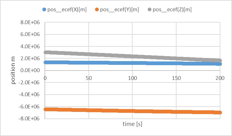
-
- results
- Calculated gravity acceleration by
gravitysphericalharmonic(r,'EGM96',360,'Error' )
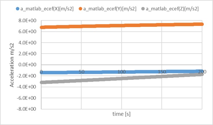
- Difference between
CalcAccelerationECEFoutput whendegree=0=1and Matlab's output (degree = 360)- You can see significant error since
CalcAccelerationECEFdoes not care about high-order gravity potential.
- You can see significant error since
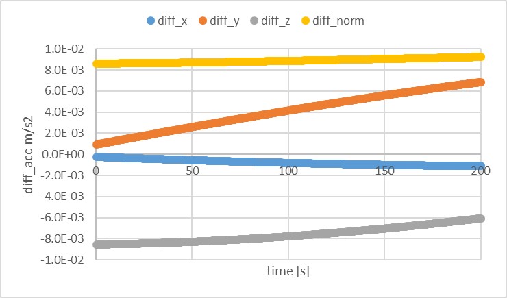
- Difference between
CalcAccelerationECEFoutput whendegree=360 and Matlab's output (degree = 360`)- The error is relatively small
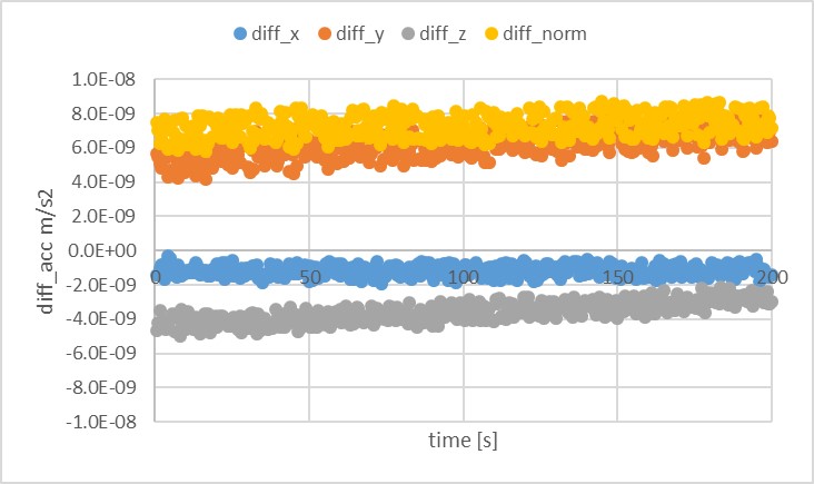
- Finally, the relationship between degree and accuracy is summarized.
- The error is limited to 1e-8 [m/s2]. The cause of the error should be considered when users need accurate orbit propagation.
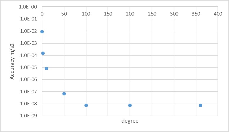
- Note
- To check the accuracy of the calculation, the resolution of
log outputshould be larger than 10.- In this case, the author chose the resolution as 15.
- To check the accuracy of the calculation, the resolution of
2. Calculation speed
1. overview
- The author has checked the relationship between the degree and the calculation speed.
chronoclass was used as follows
  chrono::system_clock::time_point start, end;
  start = chrono::system_clock::now();

  debug_pos_ecef_m_ = spacecraft.dynamics_->orbit_->GetPosition_ecef_m();
  CalcAccelerationEcef(dynamics.GetOrbit().GetPosition_ecef_m());

  end = chrono::system_clock::now();
  time_ms_ = static_cast<double>(chrono::duration_cast<chrono::microseconds>(end - start).count() / 1000.0);
- The
time_ms_is logged every log output step, and 400 data of the calculation time is saved. The averaged value of the 400 data is evaluated here. - Environment
- Core i7-8650U(2.11GHz)
- VS2017 32bit debug
2. conditions for the verification
- input files
- Same with accuracy verification
- initial values
- Same with accuracy verification
3. results
- When
degree=0=1, the calculation time is just0.018 msec. - When
degree=2 and 10, the calculation time is0.035 msec and 0.2 msec, respectively. - When
degree=360, the calculation time reaches110 msec, but it is faster than the calculation time ofgravitysphericalharmonic( r, 'EGM96',360, 'Error' ), which is700 ms.
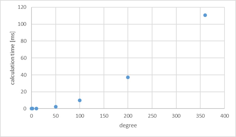
- Note
4. References
- Oliver Montenbruck, and Eberhard Gill, "Satellite Orbits", Springer
- NASA's EMG96 website
- Matlab Gravity Spherical Harmonics
- Summary of gravity models
Gravity Gradient Torque
Magnetic Disturbance Torque
Surface Force
1. Overview
1. Functions
- S2E handles air drag and Solar Radiation Pressure(SRP) as surface force disturbances since both disturbances affect spacecraft surfaces. The structure of both equations is identical, but they have different coefficients.
- Thus, the
SurfaceForcebase class provides the structure of the equation, andAirDragandSolarRadiationPressureDisturbancesubclasses provide specific calculations with appropriate coefficients. - Currently, the
SurfaceForceclass supports multi-surface spacecraft without a self-shadowing effect. Users can select the number of surfaces. - For the detailed description of
AirDragandSolarRadiationPressureDisturbance, please refer Air Drag and Solar Radiation Pressure.
2. Related files
surface_force.cpp,surface_force.hpp: The base classSurfaceForceis defined.
3. How to use
- Make a subclass that inherits the
SurfaceForceclass. - Define the
CalcCoefficientsfunction in the subclass. - Execute
CalcTorqueForcein the update function of the subclass.
2. Explanation of Algorithm
1. Constructor
1. overview
- Initialize structure parameters
2. inputs and outputs
- input
- List of
Surfaceclass which manages surface area, position, and normal direction. - Position vector of the center of gravity in the body fixed frame [m].
- List of
- output
- The instance of the class
3. algorithm: NA
4. note
- The origin of all vectors defined here is the body-fixed frame. Users can define the origin of the body-fixed frame by themselves. If users want to define the origin as the center of gravity, they need to set
center_of_gravity_b_m = zero vectorin theStructure.ini. If users want to define the origin as a specific point, they need to carefully set all vectors to suit their definition.
2. CalcTorqueForce function
1. overview
- This is the main function to calculate the force and torque generated by the surface force disturbances.
2. inputs and outputs
- input
input_direction_b: direction of disturbance source at the body frameitem: parameter which decides the magnitude of the disturbances (Solar flux, air density)- Surface information defined in the constructor
- output
force_b_N_: Force at the body frame (unit: N)torque_b_Nm_: Torque at the body frame (unit: Nm)- Both variables are defined in the
SimpleDisturbancebase class
3. algorithm
- Let us consider the following coordinate on a surface for surface force calculation
- $\boldsymbol{n}$ is the normal vector of the surface
- $\boldsymbol{v}$ is the direction vector of the disturbance source (e.g., sun direction vector or velocity vector)
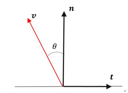
- $\boldsymbol{t}$ is the direction of in-plane force.
\[ \boldsymbol{t}=\frac{\boldsymbol{v}\times\boldsymbol{n}}{|\boldsymbol{v}\times\boldsymbol{n}|}\times\boldsymbol{n} \]
- Surface force and torque acting on the surface is expressed as following equation
- $\boldsymbol{r}_{s}$ is the position vector of the surface
- $\boldsymbol{r}_{cg}$ is the position vector of the center of mass
\[ \begin{align} \boldsymbol{F} &= -C_{n}\boldsymbol{n}+C_{t}\boldsymbol{t}\\ \boldsymbol{T} &= (\boldsymbol{r}_{s}-\boldsymbol{r}_{cg})\times\boldsymbol{F} \end{align} \]
- Detail of the $C_{n}$ and $C_{t}$ are defined by subclasses by using
CalcCoefficientsfunction
4. note
- NA
3. Results of verifications
- Verifications will be done by the subclasses.
4. References
- NA
Surface Force: Air Drag
1. Overview
1. Functions
AirDragclass inheritsSurfaceForcebase class and calculates air drag disturbance force and torque.
2. Related files
air_drag.cpp,air_drag.hpp: TheAirDragclass is defined.surface_force.cpp,surface_force.hpp: The base classSurfaceForceis defined.- Note:
SurfaceForceclass inheritsSimpleDisturbanceclass, andSimpleDisturbanceclass inheritsDisturbanceclass. So, please refer them if users want to understand the structure deeply.
- Note:
disturbance.ini: Initialization file
3. How to use
- Make an instance of the
AirDragclass inInitializeInstancesfunction indisturbances.cpp- Create an instance by using the initialization function
InitAirDrag
- Create an instance by using the initialization function
- Set the parameters in the
disturbance.ini- Select
ENABLEforcalculationandlogging - Select the following conditions of air drag calculation
- Surface Temperature degC
- Atmosphere Temperature degC
- Molecular weight of the thermosphere g/mol
- Select
2. Explanation of Algorithm
1. CalcCoefficients
1. overview
CalcCoefficientscalculates the normal and in-plane coefficients forSurfaceForcecalculation. The air drag force acting on a surface is expressed as the following equation
\[ \begin{align} \boldsymbol{F}=-C_{n}\boldsymbol{n}+C_{t}\boldsymbol{t}\\ C_{n}=\frac{1}{2}\rho A v^2 C_{n}^{\prime}\\ C_{t}=\frac{1}{2}\rho A v^2 C_{t}^{\prime} \end{align} \]
- This function mainly calculates the common part of the coefficient calculation. $C_{n}^{\prime}$ and $C_{t}^{\prime}$ are calculated in
CalCnCtfunction, and they will be used in this function.
2. inputs and outputs
- input
- $\boldsymbol{v}$: Relative velocity vector between the spacecraft and the atmosphere [m/s]
- $\rho$: air density [kg/m3]
- output
- coefficients $C_{n}$ and $C_{t}$
3. algorithm
- See above equations.
4. note: NA
2. CalCnCt
1. overview
CalCnCtcalculates $C_{n}^{\prime}$ and $C_{t}^{\prime}$.
2. inputs and outputs
- input variables
- $\boldsymbol{v}$: Relative velocity vector between the spacecraft and the atmosphere [m/s]
- Currently, we assume that this value equals spacecraft velocity in the body-fixed frame.
- $\boldsymbol{v}$: Relative velocity vector between the spacecraft and the atmosphere [m/s]
- input parameters
- $\sigma_{d}$: Diffuse coefficients for air drag
- Ini file provide specularity for air drag $\sigma_{s}$, and the diffuse coefficient is derived as $\sigma_{d}=1-\sigma_{s}$.
- Note: There is no absorption term for air drag. Thus total reflectivity is set as 1.
- $T_{w}$: Temperature of the surface [K]
- $T_{m}$: Temperature of the atmosphere [K]
- $M$: Molecular weight of the thermosphere [g/mol]
- In the default ini file, we use $M=18$, and it is a little bit smaller than the molecular weight of atmosphere $M=29$. Structure of the Thermosphere provides information on the molecular weight of the thermosphere.
- $\sigma_{d}$: Diffuse coefficients for air drag
- outputs
- $C_{n}^{\prime}$ and $C_{t}^{\prime}$
3. algorithm
- $C_{n}^{\prime}$ and $C_{t}^{\prime}$ are calculated as following equations
\[ \begin{align} C_{n}^{\prime} &= \frac{2-\sigma_{d}}{\sqrt{\pi}}\frac{\Pi(S_{n})}{S^{2}}+\frac{\sigma_{d}}{2}\frac{\chi(S_{n})}{S^{2}}\sqrt{\frac{T_{w}}{T_{m}}}\\ C_{t}^{\prime} &=\frac{\sigma_{d}}{\sqrt{\pi}}\frac{\chi(S_{n})}{S^{2}}S_{t} \end{align} \]
- $S, S_{n}, S_{t}$ are defined as follows
- $k=1.38064852E-23$ is the Boltzmann constant
- $\theta$ is the angle between the normal vector and the velocity vector
- $\cos{\theta}$ and $\sin{\theta}$ are calculated in
SurfaceForcebase class.
\[ \begin{align} S &= \sqrt{\frac{Mv^{2}}{2kT_{w}}}\\ S_{n} &= S\cos{\theta}\\ S_{t} &= S\sin{\theta}\\ \end{align} \]
- $\Pi(x)$ and $\chi(x)$ are defined as follows
- where
erfis the Gauss error function. - These functions are defined as
CalcFunctionPiandCalcFunctionChi.
- where
\[ \begin{align} \Pi(x) &= x e^{-x^{2}}+\sqrt{\pi}(x^2+0.5)(1+erf(x))\\ \chi(x) &= e^{-x^{2}}+\sqrt{\pi}x(1+erf(x)) \end{align} \]
4. note
- Please see the reference document for more information on detailed calculations.
3. Results of verifications
1. Verification of magnitude of the force
1. overview
- The calculated magnitude of the air drag force is compared with other calculation results in three cases.
2. conditions for the verification
- See the bottom table.
3. results
-
The calculation result is completely the same as the other calculation.
parameters/results Case 1 Case 2 Case 3 $\sigma_{d}$ 0.8 0.6 0.4 $\theta$ rad 0.202 0.202 0.202 $v$ m/s 7420 7420 7420 Out-plane force (S2E) 2.30297 2.68680 3.07062 Out-plane force (reference) 2.30297 2.68680 3.07062 Out-plane force (S2E) 0.31514 0.23636 0.15757 Out-plane force (reference) 0.31514 0.23636 0.15757
1. Verification of direction of the force
1. overview
- Next, we confirmed that the direction of the calculated force is correct.
2. conditions for the verification
- S2E is executed using the default setting.
3. results
- We confirmed that the direction of the force is opposite the direction of the velocity of the spacecraft.
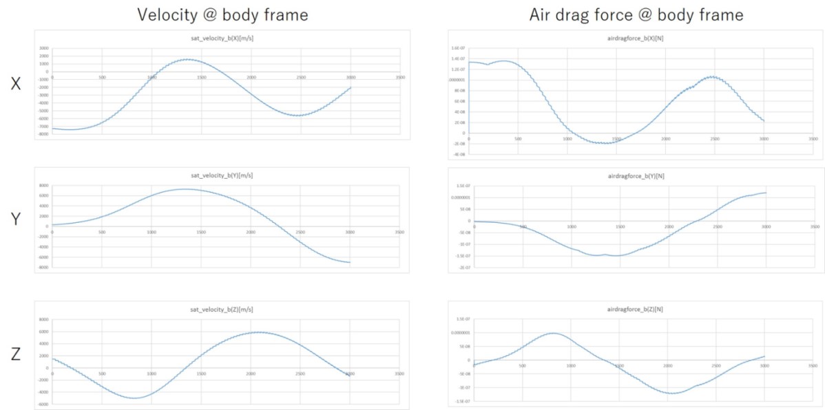
4. References
- H. Klinkrad and B. Fritsche, "ORBIT AND ATTITUDE PERTURBATIONS DUE TO AERODYNAMICS AND RADIATION PRESSURE", in ESA Workshop on Space Weather, 1998.
- Marcel Nicolet, Structure of the Thermosphere, Planetary and Space Science, 1961
- Gauss error function
Surface Force: Solar Radiation Pressure disturbance
1. Overview
1. Functions
SolarRadiationPressureDisturbanceclass inheritsSurfaceForcebase class and calculates air drag disturbance force and torque.
2. Related files
solar_radiation_pressure_disturbance.cpp,solar_radiation_pressure_disturbance.hpp: TheSolarRadiationPressureDisturbanceclass is defined.surface_force.cpp,surface_force.hpp: The base classSurfaceForceis defined.- Note:
SurfaceForceclass inheritsSimpleDisturbanceclass, andSimpleDisturbanceclass inheritsDisturbanceclass. So, please refer them if users want to understand the structure deeply.
- Note:
disturbance.ini: Initialization file
3. How to use
- Make an instance of the
SolarRadiationPressureDisturbanceclass inInitializeInstancesfunction indisturbances.cpp- Create an instance by using the initialization function
InitSolarRadiationPressureDisturbance
- Create an instance by using the initialization function
- Set the parameters in the
disturbance.ini- Select
ENABLEforcalculationandlogging
- Select
2. Explanation of Algorithm
1. CalcCoefficients function
1. overview
CalcCoefficientscalculates the normal and in-plane coefficients forSurfaceForcecalculation.
2. inputs and outputs
- inputs
- $v_{s}$:Direction vector of the sun (spacecraft to the sun) at the body frame
- $P$ Solar pressure at the position of the spacecraft [N/m^2]
- setting parameters
- $\nu$ : Total reflectance
- $\nu = 1-\alpha$, where $\alpha$ is the absorption of the sun spectrum.
- $\mu$ : Specularity. Ratio of specular reflection inside the total reflected light.
- $A$ : Area of the surface
- $\nu$ : Total reflectance
- outputs
- $C_{n}$ and $C_{t}$
3. algorithm
- $C_{n}$ and $C_{t}$ are calculated as follows:
- $\theta$ is the angle between the normal vector and the sun vector.
\[ \begin{align} C_{n} &= AP \left((1+\nu\mu)\cos^{2}{\theta}+\frac{2}{3}\nu(1-\mu)\cos{\theta} \right)\\ C_{t} &= AP(1-\nu\mu)\cos{\theta}\sin{\theta} \end{align} \]
4. note
- NA
3. Results of verifications
1. Verification of perfect reflection case
1. overview
- In the perfect reflection case, the direction of the SRP force will be opposite from the direction of the sun.
2. conditions for the verification
- We assumed that the structure of the spacecraft is a 50-cm cube whose optical property is the perfect specular reflection($\nu=\mu=1$).
3. results
- We confirmed that the direction of the SRP force is opposite from the direction of the sun at the body frame.
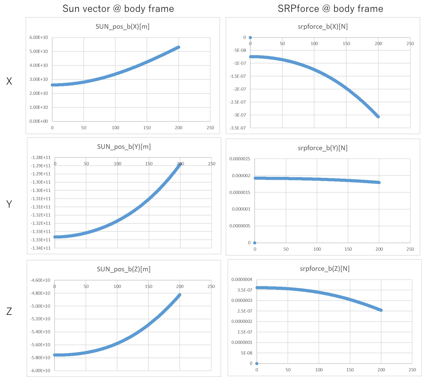
4. References
- NA
Specification of Third Body Gravity Disturbance Calculation
1. Overview
1. Functions
- The
ThirdBodyGravityclass calculates the gravity acceleration generated by the third body, such as Sun, Moon, or planets.
2. Related files
src/disturbance/third_body_gravity.cppsrc/disturbance/third_body_gravity.hpp
3. How to use
- Make an instance of the
ThirdBodyGravityclass inInitializeInstancesfunction indisturbances.cpp- Create an instance by using the initialization function
InitThirdBodyGravity
- Create an instance by using the initialization function
- Chose a orbit propagator mode that considers disturbances.
- Edit the
disturbance.inifile- Select
ENABLEforcalculationandlogging - Select
number_of_third_bodyandthird_body_nameyou need. - NOTE: All of the
third_body_nameobjects must be included in theselected_body_nameof the[CELESTIAL_INFORMATION]section in thesimulation_base.ini.
- Select
- NOTE: When the class
ThirdBodyGravityis instantiated, the class reports an error in the following cases.- The target specified by
center_objectof the[CELESTIAL_INFORMATION]section in thesimulation_base.ini. is included in the list ofthird_body. - The list of
third_body_nameincludes objects which are not in the list ofselected_body_namein the[CELESTIAL_INFORMATION]section in thesimulation_base.ini.
- The target specified by
- NOTE: If the same body is specified more than once in the list of
third_body_nameindisturbance.ini, the second and subsequent entries of the body are ignored.
2.Explanation of Algorithm
- The base algorithm is referred to Satellite Orbits chapter 3.3.
1. CalcAcceleration_i_m_s2 function
1. overview
- This function calculates the acceleration in the inertial frame generated by the third body.
2. inputs and outputs
-
Input
- position of the third body seen from the center object in the inertial coordinate system
- position of the third body seen from the spacecraft in the inertial coordinate system
- gravity constant (GM) of the third body
- NOTE: These inputs are derived from
CelestialInformation.
-
Output
- acceleration generated by the third body in the inertial coordinate system
3. algorithm
- Definition of the variables
- $\boldsymbol{r}$: the position of the spacecraft (written as
sc_position_i_min the code) - $\boldsymbol{s}$: the position of the third body (written as
third_body_pos_i_min the code) - $\boldsymbol{s}-\boldsymbol{r}$: the position of the third body seen from the spacecraft (written as
third_body_position_from_sc_i_min the code)
- $\boldsymbol{r}$: the position of the spacecraft (written as
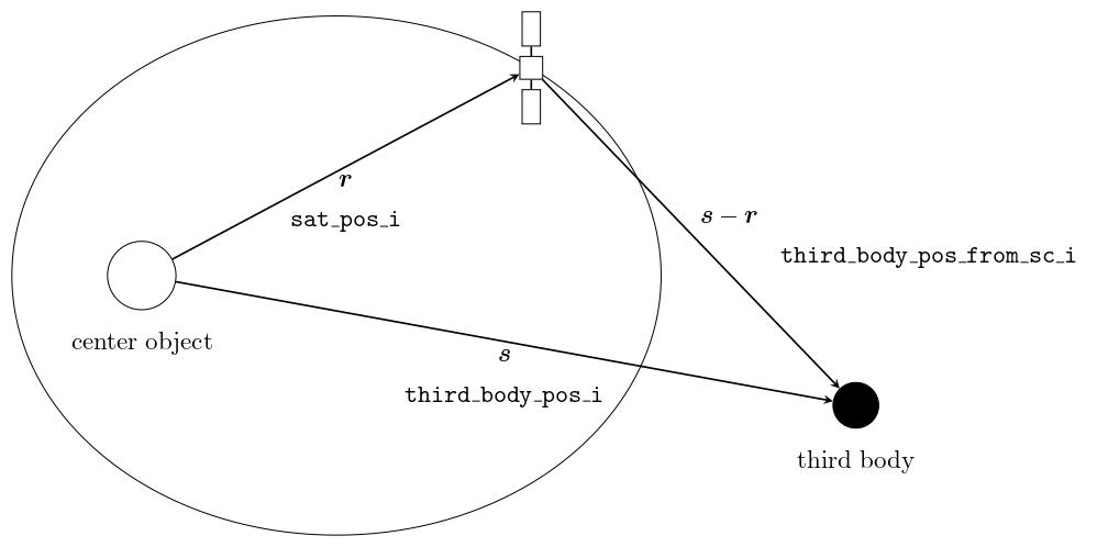
- The acceleration disturbance effect by the third body is written as follows:
\[ \ddot{\boldsymbol{r}}=GM\left(\frac{\boldsymbol{s}-\boldsymbol{r}}{|\boldsymbol{s}-\boldsymbol{r}|^3}-\frac{\boldsymbol{s}}{|\boldsymbol{s}|^3}\right) \]
- See section 3.3.1 of Satellite Orbits for a detailed explanation.
3. Results of verifications
1. overview
- The deformation of the orbit caused by the acceleration of the third body gravity is compared between S2E and STK.
2. conditions for the verification
-
input files
- Default initialize files
-
initial values
simulation_start_time_utc = 2020/01/01 11:00:00.0 simulation_duration_s = 86400 simulation_step_s = 10 orbit_update_period_s = 10 log_output_period_s = 5 simulation_speed_setting = 0-
Since the effect of third body gravity increases as one moves away from the central object, it is verified for GEO.
initial_position_i_m(0) = 42241095.67425744 initial_position_i_m(1) = 0 initial_position_i_m(2) = 0 initial_velocity_i_m_s(0) = 0 initial_velocity_i_m_s(1) = 2.978E+4 initial_velocity_i_m_s(1) = 3071.859163190527-
All the disturbance calculations, except for the third-object gravity, are set to DISABLE.
-
The following cases are tested.
- Only the gravity of the Sun is taken into account
- Only the gravity of the Moon is taken into account
- Both the gravity of the Sun and the Moon are taken into account
- Only the gravity of Mars is taken into account (TBW)
-
-
- results
- Without the third body, S2E and STK show the same result.
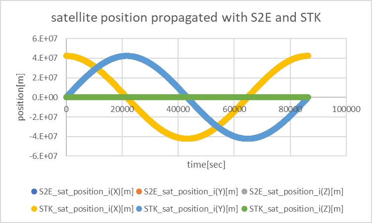
- Only the gravity of the Sun is taken into account
- The deformation of the orbit compared to GEO is shown in the following figure.
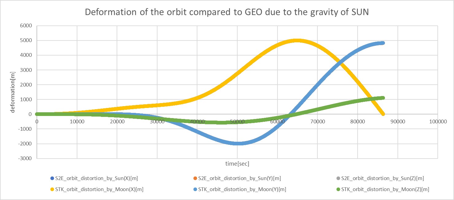
- The acceleration disturbance caused by the Sun's gravity is shown in the following figure.
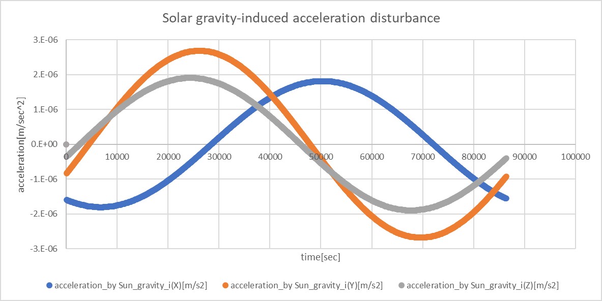
- Only the gravity of the Moon is taken into account
- The deformation of the orbit compared to GEO is shown in the following figure.
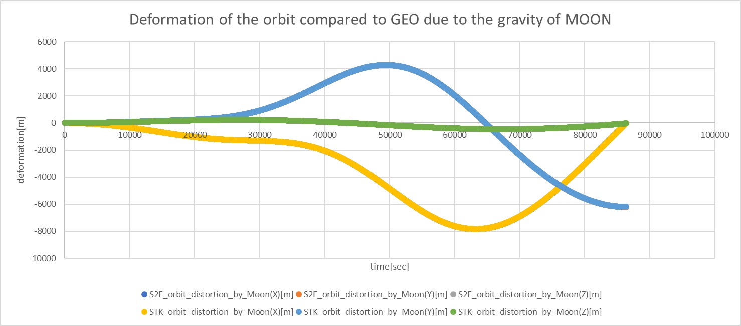
- The acceleration disturbance caused by the Moon's gravity is shown in the following figure.
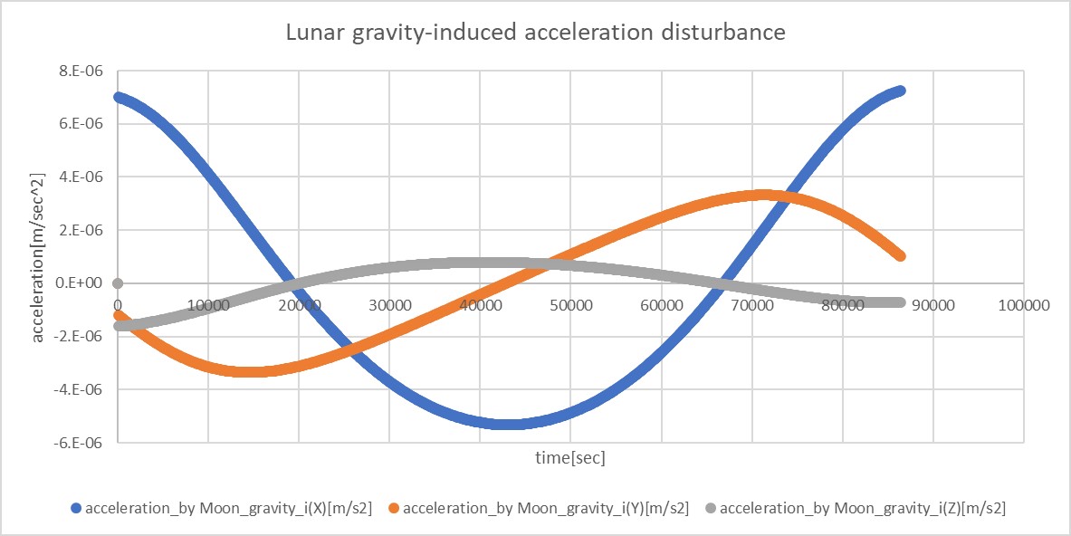
- Both the gravity of the Sun and the Moon are taken into account
- The deformation of the orbit compared to GEO is shown in the following figure.
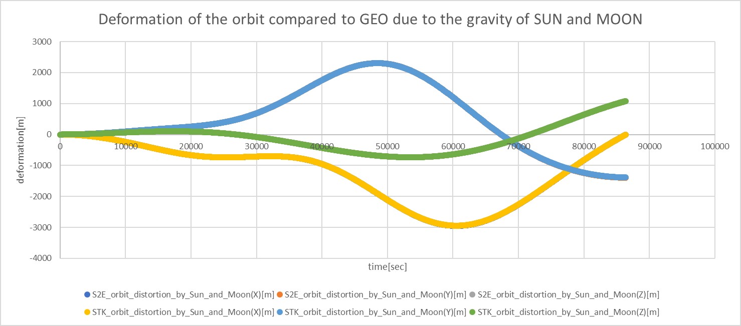
- The gravitational disturbance of both the Sun and the Moon is shown in the following figure.
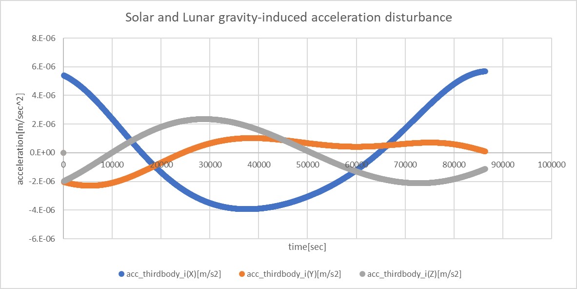
- In all of the above cases, the S2E and STK results are consistent.
4. References
- Satellite Orbits chapter 3.3.
Attitude Dynamics
Controlled Attitude
1. Overview
1. Functions
- The
ControlledAttitudeclass provides a perfectly controlled attitude instead of free motion attitude dynamics by numerical propagation. - Users can set the attitude as sun pointing, earth pointing, and others for any direction in the spacecraft body frame. Of course, users can select an inertial stabilized attitude.
- It is useful for power, communication, and orbit analyses with S2E.
2. Related files
src/dynamics/attitude/attitude.hpp, .cpp- Definition of
Attitudebase class
- Definition of
src/dynamics/attitude/controlled_attitude.hpp, .cppControlledAttitudeclass is defined here.
src/dynamics/attitude/initialize_attitude.hpp, .cpp- Make an instance of
Attitudeclass.
- Make an instance of
sample_satellite.ini: Initialization file
3. How to use
- Inside the codes
ControlledAttitudeclass inherits theAttitudeclass, so other functions can access theControlledAttitudeclass by using get functions in theAttitudeclass.
- User I/F
- Firstly, users should set
propagate_mode = CONTROLLEDat the[ATTITUDE]section in thesample_satellite.inifile. - Users can set a target attitude in the initialize file. There are the following setting parameters:
main_mode,sub_mode,initial_quaternion_i2t,pointing_t_b, andpointing_sub_t_b. - Firstly, users select the control mode by using
main_modeandsub_mode. For the control mode. - When
main_modeis set asINERTIAL_STABILIZE,sub_modeis ignored, and the spacecraft attitude is fixed to theinitial_quaternion_i2tvalue in the simulation. - When
main_modeis set asHOGE_POINTINGmodes, the direction of the body-fixed frame defined bypointing_t_bis controlled to point the specific direction of the modes.- Ex. 1, the body-fixed +X axis directs to the sun when
main_mode = SUN_POINTINGandpointing_t_b = [1.0,0.0,0.0]. - Ex. 2, the body-fixed -Z axis directs to the earth center when
main_mode = EARTH_CENTER_POINTINGandpointing_t_b = [0.0,0.0,-1.0].
- Ex. 1, the body-fixed +X axis directs to the sun when
sub_modeis only used when users selectPOINTINGmodes formain_mode.sub_modeis defined to stop rotation around the pointing direction ofmain_mode. The selected sub-direction in the body-fixed frame cannot perfectly direct the target direction since the primary target and sub-target usually do not satisfy the vertical relationship.sub_modecannot beINERTIAL_STABILIZEand the same mode withmain_mode.- The angle between
pointing_t_bandpointing_sub_t_bshould be larger than 30 degrees. (90 degrees is recommended)
- Firstly, users should set
- List of attitude control mode
- INERTIAL_STABILIZE = 0
- SUN_POINTING = 1
- EARTH_CENTER_POINTING = 2
- VELOCITY_DIRECTION_POINTING = 3
- ORBIT_NORMAL_POINTING = 4
- orbit normal $n$ is defined as $n=r\times v$, where $r$ is radial direction and $v$ is velocity direction.
2. Explanation of Algorithm
1. Initialize function
1. overview
- This function initializes the target attitude and confirms that the setting parameters are correct.
- The parameter checklist
- Out of range check for both mode definitions.
main_modeandsub_modeis not the same- The angle between
pointing_t_bandpointing_sub_t_bshould be larger than 30 degrees.
2. inputs and outputs
- NA
3. algorithm
- NA
4. note
- NA
2. Propagate function
1. overview
- This is the main function executed in every loop of attitude dynamics calculation.
2. inputs and outputs
- inputs
- setting parameters
- outputs
- quaternion_i2b
3. algorithm
- Detail algorithm is described in the next function.
4. note
- NA
3. CalcTargetDirection
1. overview
- This function calculates the target direction according to the pointing mode.
2. inputs and outputs
- inputs
- control mode
- orbit class
- celestial information class
- outputs
- the direction of the target object
3. algorithm
- As written in the code.
4. note
- NA
3. PointingCtrl
1. overview
- This function calculates the
quaternion_i2b.
2. inputs and outputs
- inputs
- the main direction of the target object in ECI frame $t_m^i$
- the sub direction of the target object in ECI frame $t_s^i$
- the main controlled direction in the body frame $d_m^b$
- the sub controlled direction in the body frame $d_s^b$
- outputs
- quaternion_i2b
3. algorithm
- Firstly, the $DCM_{t2i}$, which is the frame transformation from the target frame to the inertial frame, is calculated using $t_m^i$ and $t_s^i$ with
CalcDCM. - Next, the $DCM_{t2b}$, which is the frame transformation from the target frame to the body-fixed frame, is calculated using $d_m^b$ and $d_s^b$ with
CalcDCM. - Finally, both DCMs are combined as follows. And
quaternion_i2bis calculated from the $DCM_{i2b}$. \[ DCM_{i2b} = DCM_{t2b} \cdot DCM_{t2i}' \]
4. note
- NA
3. CalcDCM
1. overview
- This function calculates a DCM from two given directions.
- The DCM represents the coordinate transform matrix from the new frame defined by the two directions to the original frame.
2. inputs and outputs
- inputs
- the main direction in the frame $a$ : $d_m^a$
- the sub direction in the frame $a$ : $d_s^a$
- outputs
- Coordinate transform matrix from the new frame to the original frame $a$
3. algorithm
- The first basis vector of the new frame is defined as the main direction. \[ e_1=d_m^a \]
- The second basis vector needs to be direct to the sub direction, but it should be vertical with $e_1$. \[ e_2 = \frac{(e_1\times d_s^a) \times e_1}{|(e_1\times d_s^a) \times e_1|} \]
- The third basis vector is defined as right-hand coordinate. \[ e_3=\frac{e_1\times e_2}{|e_1\times e_2|} \]
4. note
- NA
3. note
- Currently, the
ControlledAttitudeclass does not calculate angular velocity, and it is set as 0. The feature will be implemented in the near future.
3. Results of verifications
1. Inertial stabilize
1. overview
- To verify the correctness of pointing control
2. conditions for the verification
- input files
- default files
- initial values
- main_mode = sub_mode = INERTIAL_STABILIZE
- initial_quaternion_i2b = [0.5,0.5,0.5,0.5]
3. results
- The inertial stabilize control is succeeded.
1. Pointing Control
1. overview
- Several cases described at the bottom were checked to verify the correctness of pointing control.
2. conditions for the verification
-
input files
- default files
-
cases
case main mode sub mode main_pointing_direction_b sub_pointing_direction_b 1 Sun Earth Center [1,0,0] [0,1,0] 2 Sun Earth Center [0,0,-1] [-1,0,0] 3 Earth Center Velocity [0,-1,0] [0,0,1] 4 Velocity Sun [0.707,0.707,0] [0,0,1]
3. results
- Case 1
- The spacecraft +X axis correctly directs to the sun, and its +Y axis roughly directs to the earth.
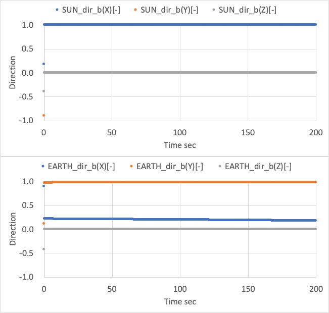
- Case 2
- The spacecraft -Z axis correctly directs to the sun, and its -X axis roughly directs to the earth.
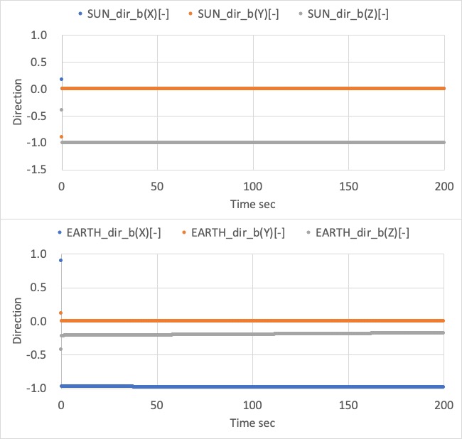
- Case 3
- The spacecraft -Y axis correctly directs to the earth, and its +Z axis roughly directs to the velocity direction.
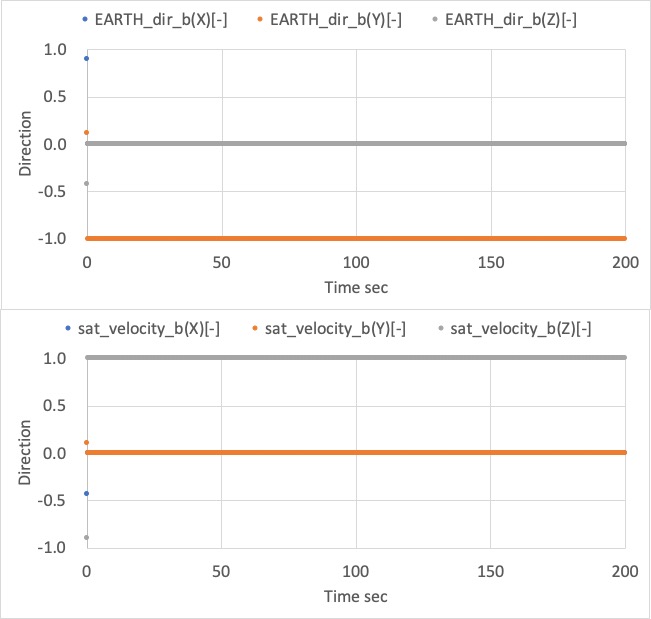
- Case 4
- The spacecraft +XY direction correctly directs to the velocity direction, and its +Z axis roughly directs to the sun.
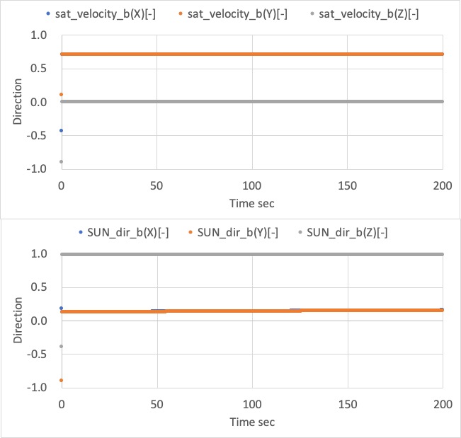
4. References
- NA
Specification for Orbit
1. Overview
1. functions
- The
Orbitclass calculates the position and velocity of satellites with the following propagation mode.KEPLER: Kepler orbit propagation without disturbances and thruster maneuverSGP4: SGP4 propagation using TLE without thruster maneuverRK4: RK4 propagation with disturbances and thruster maneuverENCKE: Encke's orbit propagation with disturbances and thruster maneuverRELATIVE: Relative dynamics (for formation flying simulation)
- The
KEPLERmode is the simplest and general for all users. - The
SGP4mode is useful for LEO satellites users without orbit control. - When users need to analyze the orbit disturbance force effect or the orbit control algorithm, the users should choose
RK4orENCKEmode. - For multiple satellite operation,
RELATIVEmode is useful.`
2. files
src/dynamics/orbit/orbit.hpp, cpp- Definition of
Orbitbase class
- Definition of
src/dynamics/orbit/initialize_orbit.hpp, .cpp- Make an instance of orbit class.
3. How to use
- Make an instance of the orbit class in
Initializefunction indynamics.cpp - Select
propagate_modein the spacecraft's ini file(eg.sample_spacecraft.ini). - Select
initialize_modein the spacecraft's ini file(eg.sample_spacecraft.ini).- This setting works only for
RK4,KEPLER, andENCKEmode.
- This setting works only for
- Set the orbit information in the ini file
- You can see the details in the documents for each orbit propagation mode.
- The definition of the coordinate system is decided at
[CELESTIAL_INFORMATION]section insample_simulation_base.ini.
2. Explanation of Algorithm
In the Orbit base class provides the following common functions for every propagator.
1. UpdateByAttitude function
- The
UpdateByAttitudefunction simply converts the velocity vector of the spacecraft (in ECI coordinate system) to body coordinate system notation using the argument:quaternion_i2b.
2. SetAcceleration_i_m_s2, AddAcceleration_i_m_s2, AddForce_i_N, AddForce_b_N function
- These functions provides the interface to include orbital disturbance or control forces.
2. TransformEcefToGeodetic function
- The
TransformEcefToGeodeticfunction calculates latitude[rad], longitude[rad], and altitude[m]. Currently, we use theGeodeticclass to calculate the information.
3. TransformEciToEcef function
- The
TransformEciToEceffunction can convert the position and the velocity of the satellite from the ECI frame to the ECEF frame, which considers the earth's rotation.
3. Results of verifications
- The verification results are described in the document of each propagation method.
4. References
NA
Specification for Kepler Orbit Propagation
1. Overview
1. Functions
- The
KeplerOrbitclass calculates the satellite position and velocity with the simple two-body problem. We ignored any disturbances and generated forces by the satellite. - This orbit propagation mode provides the simplest and fastest orbit calculation for any orbit(LEO, GEO, Deep Space, and so on.).
2. Files
src/dynamics/orbit/orbit.hpp, cpp- Definition of
Orbitbase class
- Definition of
src/dynamics/orbit/initialize_orbit.hpp, .cpp- Make an instance of orbit class.
src/dynamics/orbit/kepler_orbit_propagation.hpp, .cpp- Libraries
src/library/orbit/kepler_orbit.cpp, hppsrc/library/orbit/orbital_elements.cpp, hpp
3. How to use
- Select
propagate_mode = KEPLERin the spacecraft's ini file. - Select
initialize_modeas you want.DEFAULT: Use default initialize method (RK4andENCKEuse position and velocity,KEPLERuses init_mode_kepler)POSITION_VELOCITY_I: Initialize with position and velocity in the inertial frameORBITAL_ELEMENTS: Initialize with orbital elements
2. Explanation of Algorithm
1. KeplerOrbit::CalcConstKeplerMotion function
1. Overview
- This function calculates the following constant values.
- Mean motion
- Frame conversion matrix from in-plane position to the inertial frame position
2. Inputs and outputs
- Input
- Orbital Elements
- $\mu$ : The standard gravitational parameter of the central body
- Output
- $n$ : Mean motion
- $R_{p2i}$ : Frame conversion matrix from in-plane position to the inertial frame position
3. Algorithm
- Mean motion \[ n = \sqrt{\frac{\mu}{a^3}} \]
- Frame conversion matrix from in-plane position to ECI position \[ R_{p2i} = R_z(-\Omega)R_x(-i)R_z(-\omega) \] \[ R_x(\theta) = \begin{pmatrix} 1 & 0 & 0 \\ 0 & \cos{\theta} & \sin{\theta} \\ 0 & -\sin{\theta} & \cos{\theta} \end{pmatrix} \] \[ R_z(\theta) = \begin{pmatrix} \cos{\theta} & \sin{\theta} & 0 \\ -\sin{\theta} & \cos{\theta} & 0 \\ 0 & 0 & 1 \end{pmatrix} \]
2. KeplerOrbit::CalcOrbit function
1. Overview
- This function calculates the position and velocity of the spacecraft in the inertial frame at the designated time.
2. Inputs and outputs
- Input
- $t$ : Time in Julian day
- Orbital Elements
- Constants
- Output
- $\boldsymbol{r}_{i}$ : Position in the inertial frame
- $\boldsymbol{v}_{i}$ : Velocity in the inertial frame
3. Algorithm
- Calculate mean anomaly $l$[rad] \[ l = n * (t-t_{epoch}) \]
- Calculate eccentric anomaly $u$[rad] by solving the Kepler Equation
- Details are described in
KeplerOrbit::SolveKeplerFirstOrder
- Details are described in
- Calculate two dimensional position $x^{*}$, $y^{*}$ and velocity $\dot{x}^{*}$, $\dot{y}^{*}$ in the orbital plane \[ \begin{align} x^* &= a(\cos{u}-e)\\ y^* &= a\sqrt{1-e^2}\sin{u}\\ \dot{x}^* &= -an\frac{\sin{u}}{1^e\cos{u}}\\ \dot{y}^* &= an\sqrt{1-e^2}\frac{\cos{u}}{1^e\cos{u}}\\ \end{align} \]
- Convert to the inertial frame \[ \begin{align} \boldsymbol{r}_{i} &= R_{p2i}\begin{bmatrix} x^* \\ y^* \\ 0 \end{bmatrix}\\ \boldsymbol{v}_{i} &= R_{p2i}\begin{bmatrix} \dot{x}^* \\ \dot{y}^* \\ 0 \end{bmatrix}\\ \end{align} \]
3. KeplerOrbit::SolveKeplerFirstOrder function
1. Overview
- This function solves the Kepler Equation with the first-order iterative method.
- Note: This method is not suited to the high eccentricity orbit. It is better to use the Newton-Raphson method for such a case.
- From
v6.0.0we haveSolveKeplerNewtonMethodand use it. The detail of the method will be write.
- From
2. Inputs and outputs
- Input
- $e$ : eccentricity
- $l$ : mean anomaly [rad]
- $\epsilon$ : threshold for convergence [rad]
- Limit of iteration
- Output
- $u$ : eccentric anomaly [rad]
3. Algorithm
- Set the initial value of eccentric anomaly as follows
- $u_0=l$
- Calculate $u_{n+1}$ with the following equation \[ u_{n+1} = l + e\sin{u_n} \]
- Iterate the calculation until the following conditions are satisfied
- $|u_{n+1} - u_{n}| < \epsilon$
- The iteration number over the limit of iteration
4. OrbitalElements::CalcOeFromPosVel function
1. Overview
- This function calculates the orbital elements from the initial position and velocity in the inertial frame.
2. Inputs and outputs
- Input
- $\mu$ : The standard gravitational parameter of the central body
- $t$ : Time in Julian day
- $\boldsymbol{r}_{i}$ : Initial position in the inertial frame
- $\boldsymbol{v}_{i}$ : Initial velocity in the inertial frame
- Output
- orbital element
3. Algorithm
- $\boldsymbol{h}_{i}$ : Angular momentum vector of the orbit \[ \boldsymbol{h}_{i} = \boldsymbol{r}_{i} \times \boldsymbol{v}_{i} \]
- $a$ : Semi-major axis \[ a = \frac{\mu}{2\frac{\mu}{r} - v^2} \]
- $i$ : Inclination \[ i = \cos^{-1}{h_z} \]
- $\Omega$ : Right Ascension of the Ascending Node (RAAN)
- Note: This equation is not support $i = 0$ case. \[ \Omega = \sin^{-1}\left(\frac{h_x}{\sqrt{h_x^2 + h_y^2}}\right) \]
- $x_{p}, y_{p}$ : Position in the orbital plane \[ \begin{align} x_{p} &= r_{ix} \cos{\Omega} + r_{iy} \sin{\Omega};\\ y_{p} &= (-r_{ix} \sin{\Omega} + r_{iy} \cos{\Omega})\cos{i} + r_{iz}\sin{i} \end{align} \]
- $\dot{x}_{p}, \dot{y}_{p}$ : Velocity in the orbital plane \[ \begin{align} \dot{x}_{p} &= v_{ix} \cos{\Omega} + v_{iy} \sin{\Omega};\\ \dot{y}_{p} &= (-v_{ix} \sin{\Omega} + v_{iy} \cos{\Omega})\cos{i} + v_{iz}\sin{i} \end{align} \]
- $e$ : Eccentricity \[ \begin{align} c_1 &= \frac{h}{\mu}\dot{y}_p - \frac{x_p}{r}\\ c_2 &= -\frac{h}{\mu}\dot{x}_p - \frac{y_p}{r}\\ e &= \sqrt{c_1^2 + c_2^2} \end{align} \]
- $\omega$ : Argument of Perigee \[ \omega = \tan^{-1}\left(\frac{c_2}{c_1}\right) \]
- $t_{epoch}$ : Epoch [Julian day] \[ \begin{align} f &= \tan^{-1}\left(\frac{y_p}{x_p}\right) - \omega\\ u &= \tan^{-1}\frac{\frac{r \sin{f}}{\sqrt{1-e^2}}}{r\cos{f} + ae}\\ \end{align} \] \[ \begin{align} n &= \sqrt{\frac{\mu}{a^3}}\\ dt &= \frac{u - e\sin{u}}{n}\\ t_{epoch} &= t - \frac{dt}{246060} \end{align} \]
3. Results of verifications
1. Comparison with RK4
1. Overview
- We compared the calculated orbit result between RK4 mode and Kepler mode. In the RK4 mode, all disturbances are disabled since the Kepler mode ignores them.
- In the Kepler mode, we verified the correctness of both initialize modes (
ORBITAL_ELEMENTSandPOSITION_VELOCITY_I).
2. Conditions for the verification
- sample_simulation_base.ini
- The following values are modified from the default.
EndTimeSec = 10000
LogOutPutIntervalSec = 5
- The following values are modified from the default.
- SampleDisturbance.ini
- All disturbances are disabled.
- SampleSat.ini
- The following values are modified from the default.
propagate_modeis changed for each mode.- Orbital elements for Kepler
semi_major_axis_m = 6794500.0 eccentricity = 0.0015 inclination_rad = 0.9012 raan_rad = 0.1411 arg_perigee_rad = 1.7952 epoch_jday = 2.458940966402607e6 - Initial position and velocity (compatible value with the orbital elements)
init_position(0) = 1791860.131
init_position(1) = 4240666.743
init_position(2) = 4985526.129
init_velocity(0) = -7349.913889
init_velocity(1) = 631.6563971
init_velocity(2) = 2095.780148
- The following values are modified from the default.
3. Results
-
The following figure shows the orbit calculation result of Kepler mode with
ORBITAL_ELEMENTSinitialize mode.- The result looks correct.
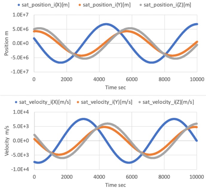
-
The difference between Kepler mode with
ORBITAL_ELEMENTSinitialize mode and RK4 mode is shown in the following figure.- The error between them is small (less than 10m), and we confirmed that the calculation of Kepler orbit is correct.
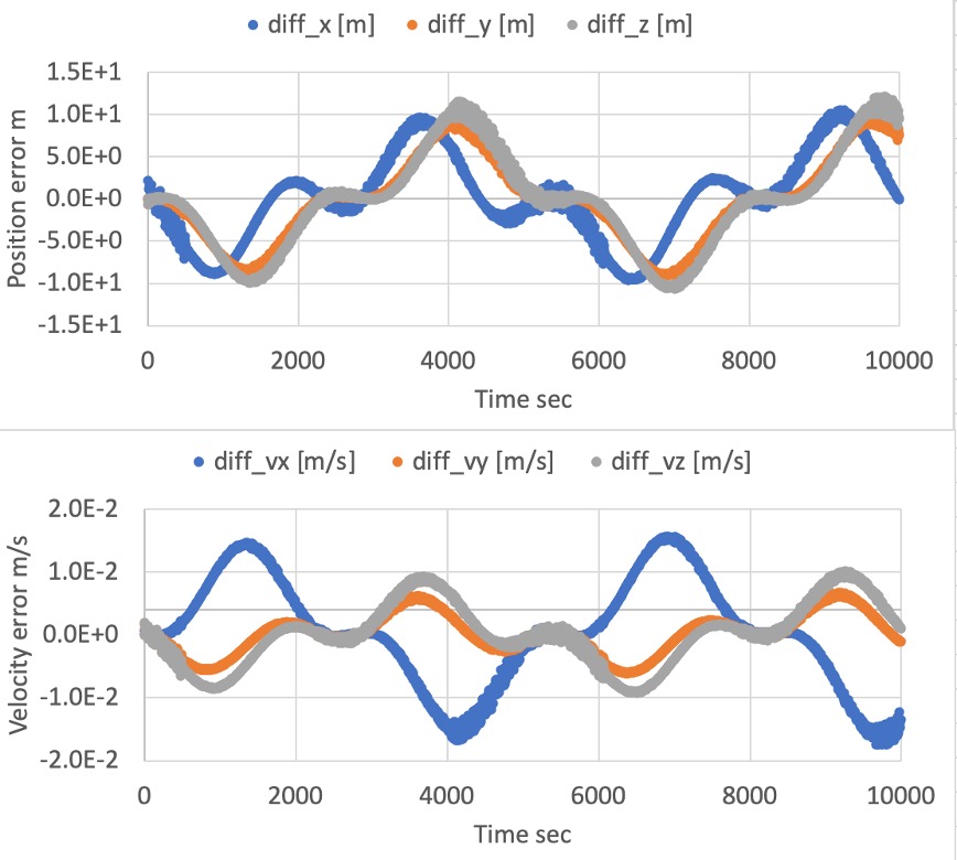
-
The following figure shows the difference between Kepler orbit calculation with
ORBITAL_ELEMENTSandPOSITION_VELOCITY_Iinitialize mode.- The error between them is small (less than 10m), and we confirmed that the initializing method is correct.
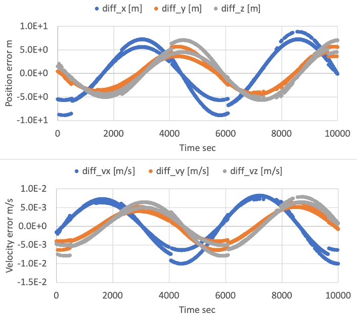
4. References
- Hiroshi Kinoshita, "Celestial mechanisms and orbital dynamics", ch.2, 1998 (written in Japanese)
Specification for SGP4 Orbit Propagation
1. Overview
1. functions
- The
Sgp4OrbitPropagationclass calculates the position and velocity of satellites by using SGP4 method with TLE.
2. files
src/dynamics/orbit/orbit.hpp, cpp- Definition of
Orbitbase class
- Definition of
src/dynamics/orbit/initialize_orbit.hpp, .cpp- Make an instance of orbit class.
src/dynamics/orbit/sgp4_orbit_propagation.hpp, .cpp- Library of SGP4
/src/library/external/sgp4
3. How to use
- Select
propagate_mode = SGP4in the spacecraft's ini file. - Set the TLE you need like the following example
tle1=1 25544U 98067A   20076.51604214  .00016717  00000-0  10270-3 0  9005
tle2=2 25544  51.6412  86.9962 0006063  30.9353 329.2153 15.49228202 17647
2. Explanation of Algorithm
1. Propagate function
- The difference between the
current Julian dayand the original period in TLE in units of [minutes] (elapse_time_min) is calculated, and it is used in the argument of the sgp4 function of the SGP4 calculation execution function. At the same time, the geodetic system definition (whichconst) and the trajectory information structure (satrec) are also required, which are defined at the call of the constructor. The position [m] and velocity [m/s] of the spacecraft are assigned to the member variables sat_position_i_ and sat_velocity_i_ as the output of the sgp4 function. Note that the values, in this case are the values from the ECI coordinate system.
3. Results of verifications
1. Verification of SGP4
1. Overview
- Verify whether the propagation of SGP4 is correctly installed or not.
- By comparing the propagation result of SGP4 in STK simulator and S2E
2. Conditions for the verification
- Conduct verification using the two different initial TLE cases with different time spans.
-
Hodoyoshi orbit : (span:10000 second)
- TLE
40299U 14070B 20001.00000000 -.00003285 00000-0 -13738-3 0 00007 40299 097.3451 081.6192 0014521 069.5674 178.3972 15.23569636286180 -
ISS Release orbit (span:10 days)
- TLE
99999U   20001.00000000  .00000007  00000-0  93906-7 0 00002
99999 053.4260 297.1689 0008542 245.4975 274.8981 15.55688139000015
3. Results
-
Hodoyoshi orbit : (span:10000 second)
- Left: STK, Right: S2EThe outputs of the satellite position are almost the same between the two simulators.
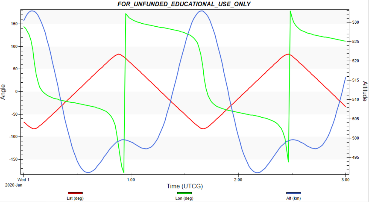
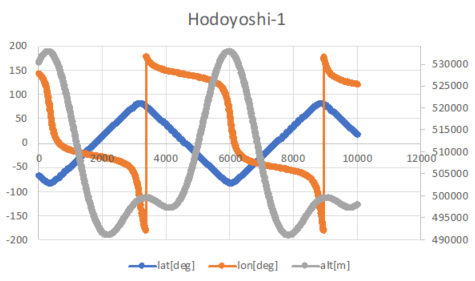
- Left: STK, Right: S2E
-
ISS Release orbit : (span:10000 second)
- Left: STK, Right: S2E The outputs of the satellite position are almost the same between the two simulators.
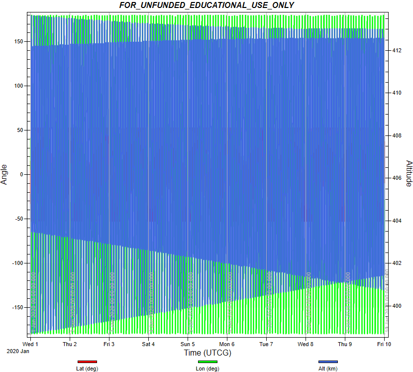
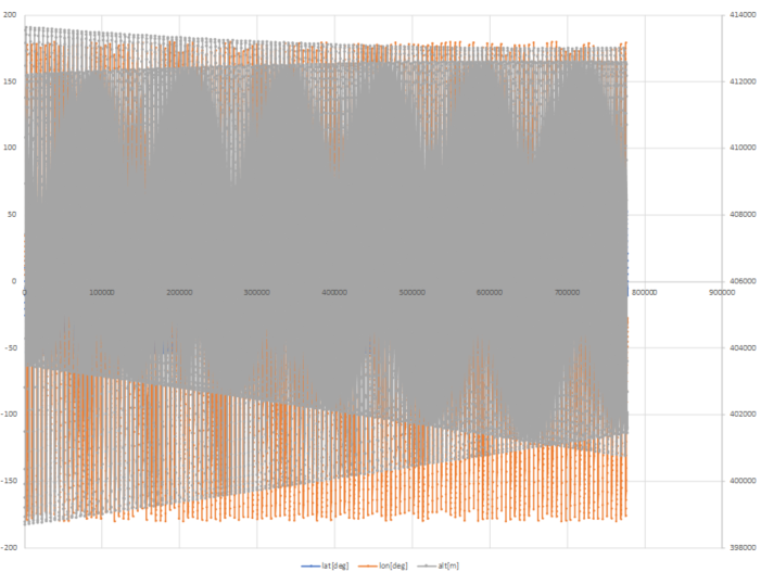
- Left: STK, Right: S2E
4. References
NA
Specification for Orbit dynamics with RK4 propagation
1. Overview
1. functions
- The
Rk4OrbitPropagationclass calculates the position and velocity of satellites with 4th Order Runge-Kutta method(RK4).
2. files
src/dynamics/orbit/orbit.hpp, cpp- Definition of
Orbitbase class
- Definition of
src/dynamics/orbit/initialize_orbit.hpp, .cpp- Make an instance of orbit class.
src/dynamics/orbit/rk4_orbit_propagation.hpp, .cpp
3. How to use
- Select
propagate_mode = RK4in the spacecraft's ini file. - Select
initialize_modeas you want.DEFAULT: Use default initialize method (RK4andENCKEuse position and velocity,KEPLERuses init_mode_kepler)POSITION_VELOCITY_I: Initialize with position and velocity in the inertial frameORBITAL_ELEMENTS: Initialize with orbital elements
2. Explanation of Algorithm
1. Propagate function
- The position and velocity of the satellite are updated by using RK4. As the input of RK4, the six-state variables are set. These state variables are the three-dimensional position [$x$, $y$ ,$z$] and three-dimensional velocity [$v_x$, $v_y$, $v_z$] at the inertial coordinate. Here, the inertial coordinate is decided by the
PlanetSelect.ini - As the force which works to the satellite motion is the external acceleration [$a_x$,$a_y$,$a_z$] calculated from the disturbance class or thruster class and the gravity force from the center planet, which is defined in
PlanetSelect.ini. As a summary, the orbit is calculated as the following equation. \[ \begin{align} \dot{x} &= v_x\\ \dot{y} &= v_y\\ \dot{z} &= v_z\\ \dot{v}_x &= a_x-\mu\frac{x}{r^3}\\ \dot{v}_y &= a_y-\mu\frac{y}{r^3}\\ \dot{v}_z &= a_z-\mu\frac{z}{r^3}\\ r &= \sqrt{x^2+y^2+z^2} \end{align} \]
3. Results of verifications
1. Verification of the error of Fourth Order Runge-Kutta method (RK4)
1. Overview
- Verify the numerical integration error of the RK4 method.
- The output of the simulation was compared with the analytical solution.
2. conditions for the verification
- The Verifications were conducted in the case of
simulation_step_sandorbit_update_period_swere 0.1(sec), 1(sec), and 10(sec). - The initial values of the propagation are as follows:
initial_position_i_m(0) = 1.5944017672e7 initial_position_i_m(1) = 0.0 initial_position_i_m(2) = 0.0 initial_velocity_i_m_s(0) = 0.0 initial_velocity_i_m_s(1) = 5000.0 initial_velocity_i_m_s(2) = 0.0 - This is a circular orbit, which period is about 20040(sec). The center of the orbit is Earth.
- As a reference, the analytical solution was used. The solution is as follows: \[ x=R\cos(\omega t),y=R\sin(\omega t)\quad when~R=1.5944017672\times10^7, \omega=0.000313597243985794 \]
- All of the effects of disturbance and environment were disabled.
- The simulation time is 60120(sec), which is approximately three-period. In addition, for a long-term test, the case in which simulation time is 200400(about 10 periods) was tested. The
orbit_update_period_sof this case is 1(sec).
3. results
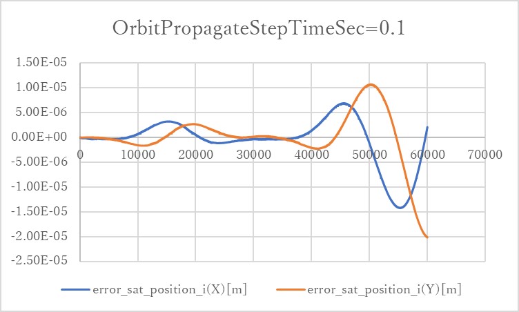
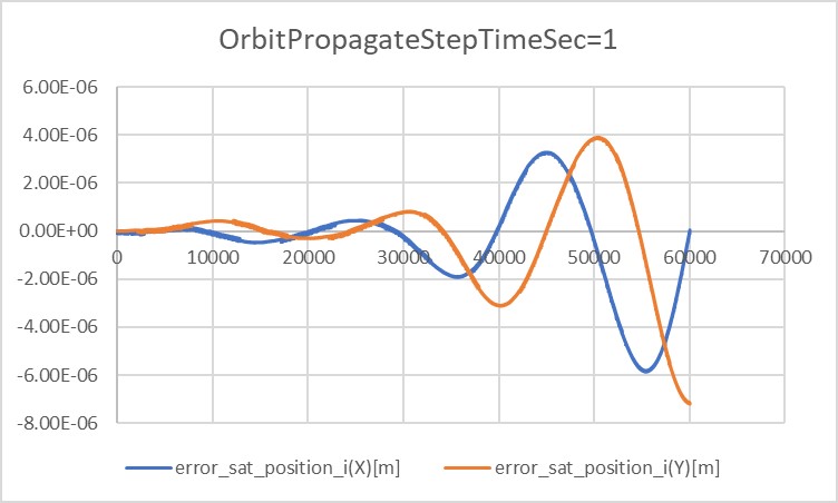
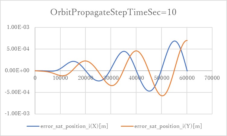
- In the cases of
orbit_update_period_s=0.1andorbit_update_period_s=1, the error is kept within $10^{-6}$ order. However, once the error grows, it will get bigger and bigger. - In the case of
orbit_update_period_s=10, the error quickly grows up to $10^{-4}$ order.
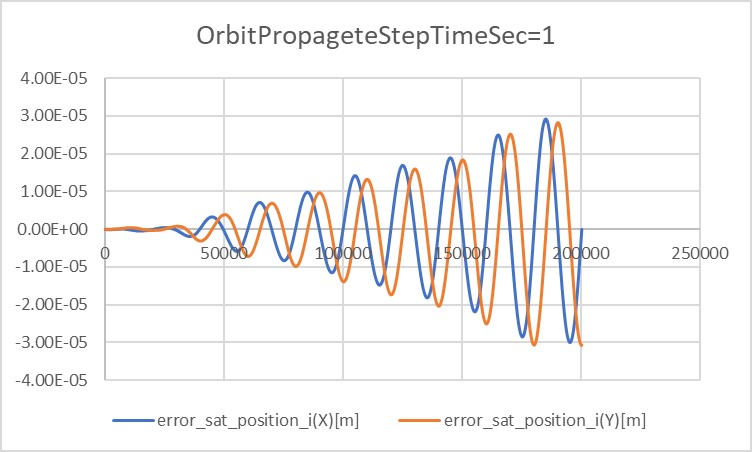
- In the long-term test result, it is clear that the error magnitude grows proportionally to the time.
4. Others
- At first, the output of STK would be used for reference. However, it did not work well. Data were input as follows:
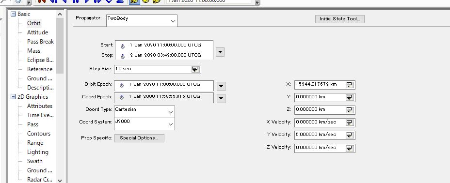
- However, the result is as follows:
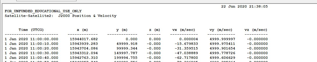
- As this figure shows, the initial values in the result are slightly different from the input.
- In the .sa files, the initial values of $x, y, z, v_x, v_y, v_z$ are converted into elements of orbit and stored. The error might occur in the process of this conversion.
4. References
NA
Specification for Orbit Propagation with Encke's Method
1. Overview
1. functions
- The
EnckeOrbitPropagationclass calculates the satellite position and velocity with Encke's method, including disturbances and controlled accelerations by the satellite. - This orbit propagation mode provides an accurate and efficient orbit calculation with disturbance forces.
- We can also use it for accurate relative orbit propagation, and the feature will be implemented soon.
2. files
src/dynamics/orbit/orbit.hpp, cpp- Definition of
Orbitbase class
- Definition of
src/dynamics/orbit/initialize_orbit.hpp, .cpp- Make an instance of orbit class.
src/dynamics/orbit/encke_orbit_propagation.cpp, .hpp- We use KeplerOrbit libraries to calculate the reference orbit.
3. How to use
- Select
propagate_mode = ENCKEin the spacecraft's ini file. - Select
initialize_modeas you want.DEFAULT: Use default initialize method (RK4andENCKEuse position and velocity,KEPLERuses init_mode_kepler)POSITION_VELOCITY_I: Initialize with position and velocity in the inertial frameORBITAL_ELEMENTS: Initialize with orbital elements
- Set the value of
error_tolerance, which decides the threshold for the rectification.
2. Explanation of Algorithm
1. EnckeOrbitPropagation::Initialize function
1. Overview
- This function generates the initial value of the reference orbit and the difference orbit.
2. Inputs and outputs
- Input
- $\mu$ : The standard gravitational parameter of the central body
- $t$ : Time in Julian day
- $\boldsymbol{r}_{i}$ : Initial position in the inertial frame
- $\boldsymbol{v}_{i}$ : Initial velocity in the inertial frame
- Output
- The reference orbit
- The difference is set as zero
3. Algorithm
- The reference orbit is initialized as the Kepler Orbit with
OrbitalElements::CalcOeFromPosVelfunction. The detail of the function is described in Specification for Kepler Orbit Propagation
2. EnckeOrbitPropagation::Propagate function
1. Overview
- This function is the main algorithm of Encke's method and calculates the orbit of the spacecraft.
- The method separates the orbit to the reference and the difference. The reference is calculated with the Kepler orbit method as a two-body problem, and the difference is calculated, including the disturbances.
- $\boldsymbol{r}_{ref}$ : Reference orbit
- $\boldsymbol{\delta}$ : Difference
- Please refer to the references to learn the original idea of Encke's method.
2. Inputs and outputs
- Input
- $\boldsymbol{a}_d$ : Acceleration
- $t$ : Current time
- Output
- $\boldsymbol{r}_{i}$ : Initial position in the inertial frame
- $\dot{\boldsymbol{r}}_{i}$ : Initial velocity in the inertial frame
3. Algorithm
- Rectification
- If the norm of the difference is larger than the tolerance, we need to update the reference orbit as the latest orbit information.
- Update reference orbit
- The reference orbit is calculated with the Kepler orbit calculation method.
- Propagate the difference
- Propagate the following differential equation. At this moment, we use the fourth-order Runge-Kutta method as a propagator. \[ \begin{align} \ddot{\boldsymbol{\delta}} &= -\frac{\mu}{r_{ref}^3}(\boldsymbol{\delta}+f(q)\boldsymbol{r})+\boldsymbol{a}_d\\ f(q) &= q \frac{q^2 + 3q + 3}{(1+q)^{1.5} + 1}\\ q &= \frac{\boldsymbol{\delta}\cdot(\boldsymbol{\delta}-2\boldsymbol{r}_i)}{r_i} \end{align} \]
3. Results of verifications
1. Comparison with RK4
1. Overview
- We compared the calculated orbit result between RK4 mode and Kepler mode.
- In the Kepler mode, we verified the correctness of both initialize mode (
ORBITAL_ELEMENTSandPOSITION_VELOCITY_I).
2. Conditions for the verification
- sample_simulation_base.ini
- The following values are modified from the default.
EndTimeSec = 10000
LogOutPutIntervalSec = 5
- The following values are modified from the default.
- SampleDisturbance.ini
- The disturbance setting is depending on the simulation case.
- All disabled or enabled. Other settings are default.
- The disturbance setting is depending on the simulation case.
- SampleSat.ini
- The following values are modified from the default.
propagate_modeis changed for each mode.- Orbital elements for Kepler
semi_major_axis_m = 6794500.0 eccentricity = 0.0015 inclination_rad = 0.9012 raan_rad = 0.1411 arg_perigee_rad = 1.7952 epoch_jday = 2.458940966402607e6 - Initial position and velocity (compatible value with the orbital elements)
initial_position_i_m(0) = 1791860.131
initial_position_i_m(1) = 4240666.743
initial_position_i_m(2) = 4985526.129
initial_velocity_i_m_s(0) = -7349.913889
initial_velocity_i_m_s(1) = 631.6563971
initial_velocity_i_m_s(2) = 2095.780148
- The following values are modified from the default.
- Results
-
The following figure shows the difference between orbit derived with Kepler mode initialized with OE and Encke mode without any disturbances.
- The error is small (less than 10m), and we confirmed that the Encke propagation mode is correct when the disturbances are zero.
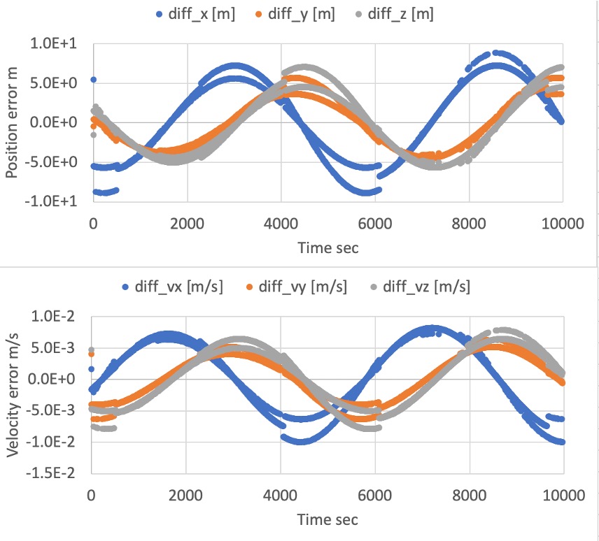
-
The following figure shows the difference between orbit derived with RK4 mode and Encke mode with all disturbances.
- The error is larger than the non-disturbance case, but the $10^4 [m]$ error between the Encke method and the Cowell method is compatible with the ref[2] when using the RK4 in LEO. We confirmed that the Encke propagation mode is correct when all disturbances are included.
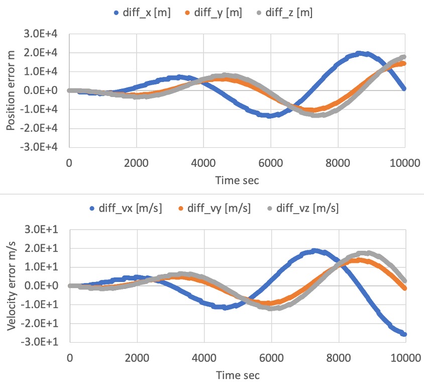
4. References
- [1] David A. Vallado, "Fundamental of Astrodynamics and Applications, Third Edition", ch.8, 2007.
- [2] Simon P. Shuster, "A Survey and Performance Analysis of Orbit Propagators for LEO, GEO, and Highly Elliptical Orbits", 2017.
Specification for Relative Orbit propagation
1. Overview
1. functions
- The
RelativeOrbitclass calculates the position of a satellite with respect to a reference satellite. This class calculates the position both in the LVLH frame and inertial frame. Users can choose the update method between:- relative dynamics propagation using RK4
- update using STM(State Transition Matrix)
2. Related files
src/dynamics/orbit/orbit.hpp, cpp- Definition of
Orbitbase class
- Definition of
src/dynamics/orbit/initialize_orbit.hpp, .cpp- Make an instance of orbit class.
src/dynamics/orbit/relative_orbit.hpp, .cpp- Definition of the class
- Libraries
src/library/orbit/relative_orbit_models.hpp, .cpp
- Library to store equations for various relative dynamics
3. How to use
-
Relative orbit propagation is available only when multiple satellites are simulated.
- The sample case in S2E_CORE simulates a single satellite. For an example of simulating multiple satellites, please refer to the tutorial.
-
Confirm the instance of
RelativeInformationis the member of each satellite. -
Set up the configuration of the
[ORBIT]section in thesample_spacecraft.ini.- Set
propagate_mode = RELATIVEto use the relative orbit propagation - Choose
relative_orbit_update_method.relative_orbit_update_method = 0means the orbit is updated with the propagation of the relative dynamics equation( $\dot{\boldsymbol{x}}=\boldsymbol{Ax}+\boldsymbol{Bu}$ , i.e., Hill equation).relative_orbit_update_method = 1means the orbit is updated with the STM( $\boldsymbol{x}(t)=\boldsymbol{\Phi}(t,t_0)\boldsymbol{x}(t_0)$ , i.e., Clohessy-Wiltshire solution).
- When you choose
relative_orbit_update_method = 0, setrelative_dynamics_model_type. - When you choose
relative_orbit_update_method = 1, setstm_model_type. - Set the initial relative position of the satellite in the LVLH frame. LVLH frame definition is:
- $\boldsymbol{x}$ is a direction vector from the reference satellite ("chief" in the figure) radially outward.
- The direction of $\boldsymbol{z}$ corresponds to the angular momentum vector of the reference satellite orbit.
- The direction of $\boldsymbol{y}$ is determined by $\boldsymbol{z}\times\boldsymbol{x}$.
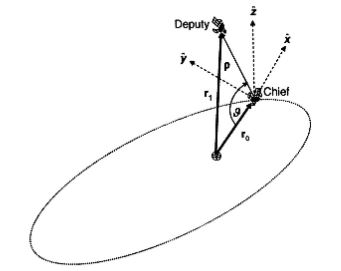
Definition of LVLH frame [1] - Set the ID and ini file name of the reference satellite.
- NOTE: Confirm the
propagate_modeof the reference satellite is not 2. The orbit of the reference satellite must be propagated by the methods other than the relative orbit propagation.
- NOTE: Confirm the
- Set
4. How to add a new relative dynamics model
- New Relative Dynamics equation
- Add the name of the dynamics model to the
RelativeOrbitModelenum inrelative_orbit_models.hpp. - Add the function to calculate the system matrix like
CalcHillSystemMatrixinrelative_orbit_models.hpp. - Edit the
CalculateSystemMatrixfunction inrelative_orbit.hpp.
- New STM
- Add the name of the dynamics model to
StmModelenum inrelative_orbit_models.hpp. - Add the function to calculate the system matrix as
CalcHcwStminrelative_orbit_models.hpp. - Edit the
CalculateStmfunction inrelative_orbit.hpp.
2. Explanation of Algorithm
1. InitializeState
1. overview
- The
InitializeStatefunction initializes the orbit of the satellite.
2. inputs and outputs
- input
relative_position_lvlh_m,relative_velocity_lvlh_m_s
- The initial state of the satellite
gravity_constant_m3_s2- The gravity constant of the reference celestial body $\mu$
initial_time_s- Initial simulation time (default value is 0)
- output
- none
3. algorithm
4. note
2. CalculateSystemMatrix
1. overview
- The
CalculateSystemMatrixfunction is used only inside theRelativeOrbitclass. This function calls the system matrix calculation function according torelative_dynamics_model_type.
2. inputs and outputs
- input
relative_dynamics_model_type- The type of relative dynamics model
reference_sat_orbit- The orbit of the reference satellite
gravity_constant_m3_s2- The gravity constant $\mu$
- output
- none
3. algorithm
4. note
3. CalculateStm
1. overview
- The
CalculateStmfunction is used only inside theRelativeOrbitclass. This function calls the system matrix calculation function according tostm_model_type.
2. inputs and outputs
- input
stm_model_type- The type of relative dynamics model
reference_sat_orbit- The orbit of the reference satellite
gravity_constant_m3_s2- The gravity constant $\mu$
elapsed_sec- Elapsed simulation time
- output
- none
3. algorithm
4. note
4. CalculateHillSystemMatrix
1. overview
- The
CalculateHillSystemMatrixfunction calculates the system matrix of the Hill equation. - This function is declared in
relative_orbit_models.hppand is used by the
2. inputs and outputs
- input
orbit_radius- Radius of the reference satellite orbit $R$
gravity_constant_m3_s2- The gravity constant $\mu$
- output
system_matrix- system matrix
3. algorithm
- The mean motion of the reference orbit ($n$) is calculated as follows:
\[ n=\sqrt{\frac{\mu}{R^3}} \]
- Then, the system matrix ($\boldsymbol{A}$) is calculated as follows:
\[ \boldsymbol{A}= \begin{pmatrix} 0 & 0 & 0 & 1 & 0 & 0 \\ 0 & 0 & 0 & 0 & 1 & 0 \\ 0 & 0 & 0 & 0 & 0 & 1 \\ 3n^2 & 0 & 0 & 0 & 2n & 0 \\ 0 & 0 & 0 & -2n & 0 & 0 \\ 0 & 0 & -n^2 & 0 & 0 & 0 \\ \end{pmatrix} \]
4. note
5. CalculateHcwStm
1. overview
- The
CalculateHcwStmfunction calculates the Hill-Clohessy-Wiltshire STM. - This function is declared in
relative_orbit_models.hppand is used by the
2. inputs and outputs
- input
orbit_radius- Radius of the reference satellite orbit $R$
gravity_constant_m3_s2- The gravity constant $\mu$
elapsed_sec- Elapsed simulation time
- output
system_matrix- system matrix
3. algorithm
- The mean motion of the reference orbit ($n$) is calculated as follows:
\[ n=\sqrt{\frac{\mu}{R^3}} \]
- Then, the system matrix ($\boldsymbol{A}$) is calculated as follows:
\[ \boldsymbol{\Phi}(t,t0)= \begin{pmatrix} 4-3\cos(nt) & 0 & 0 & \frac{\sin(nt)}{n} & \frac{2}{n}-\frac{2\cos(nt)}{n} & 0 \\ -6nt+6\sin(nt) & 1 & 0 & -\frac{2}{n}+\frac{2\cos(nt)}{n} & \frac{4\sin(nt)}{n}-3t & 0 \\ 0 & 0 & \cos(nt) & 0 & 0 & \frac{\sin(nt)}{n} \\ 3n\sin(nt) & 0 & 0 & cos(nt) & 2\sin(nt) & 0 \\ -6n+6n\cos(nt) & 0 & 0 & -2\sin(nt) & -3+4\cos(nt) & 0 \\ 0 & 0 & -n\sin(nt) & 0 & 0 & \cos(nt) \\ \end{pmatrix} \]
4. note
3. Results of verifications
1. Relative Orbit Propagation
1. overview
- Make sure the relative orbit is correctly propagated using a simple orbit
2. conditions for the verification
- input files
- Initialization files for the two satellites were prepared.
satellite0.inisatellite1.ini
- Initialization files for the two satellites were prepared.
- initial values
-
The orbit of the reference satellite (satellite0) is GEO. The initial position of the satellite (satellite1) is $(0\mathrm{m}, 100\mathrm{m}, 0\mathrm{m})^\mathrm{T}$ in LVLH frame. The orbit was propagated for 86400 sec (the period of GEO).
-
satellite0.inipropagate_mode = RK4 //Information used for orbital propagation by the Runge-Kutta method/////////// //initial satellite position[m] //*The coordinate system is defined in PlanetSelect.ini initial_position_i_m(0) = 4.2164140100E+07 //radius of GEO initial_position_i_m(1) = 0 initial_position_i_m(2) = 0 //initial satellite velocity[m/s] //*The coordinate system is defined in PlanetSelect.ini initial_velocity_i_m_s(0) = 0 initial_velocity_i_m_s(1) = 3.074661E+03 //Speed of a spacecraft in GEO initial_velocity_i_m_s(2) = 0 /////////////////////////////////////////////////////////////////////////////// -
satellite1.inipropagate_mode = RELATIVE //Information used for relative orbit propagation////////////////////////////// //Relative Orbit Update Method (0 means RK4, 1 means STM) relative_orbit_update_method = 0 // RK4 Relative Dynamics model type (only valid for RK4 update) // 0: Hill relative_dynamics_model_type = 0 // STM Relative Dynamics model type (only valid for STM update) // 0: HCW stm_model_type = 0 // Initial satellite position relative to the reference satellite in LVLH frame[m] // * The coordinate system is defined at [PLANET_SELECTION] in SampleSimBase.ini initial_relative_position_lvlh_m(0) = 0.0 initial_relative_position_lvlh_m(1) = 100.0 initial_relative_position_lvlh_m(2) = 0.0 // initial satellite velocity relative to the reference satellite in LVLH frame[m/s] initial_relative_velocity_lvlh_m_s(0) = 0.0 initial_relative_velocity_lvlh_m_s(1) = 0.0 initial_relative_velocity_lvlh_m_s(2) = 0.0 // information of reference satellite reference_satellite_id = 0 ///////////////////////////////////////////////////////////////////////////////
-
3. results
- The position of satellite1 seen from satellite0 in the inertia frame was calculated.
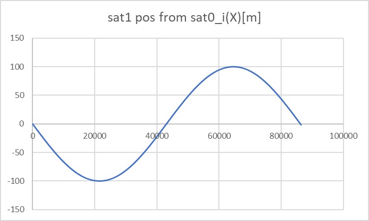
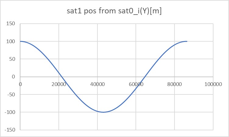
- They correctly move periodically.
- In this example of verification, the RK4 method is used to propagate relative orbits, but the results were the same when using STM.
4. References
- Kapila, V., Sparks, A. G., Buffington, J. M., & Yan, Q. (2000). Spacecraft formation flying: Dynamics and control. Journal of Guidance, Control, and Dynamics, 23(3), 561-564.
Specification for Solar Radiation Pressure Environment
1. Overview
1. Functions
SolarRadiationPressureEnvironmentcalculates solar power flux at the spacecraft's position, including the earth's eclipse effect.
2. Related files
src/environment/local/solar_radiation_pressure_environment.cpp, .hppSolarRadiationPressureEnvironmentclass is defined.
src/environment/local/local_environment.cpp, .hppSolarRadiationPressureEnvironmentclass is used here as a member variable ofLocalEnvironmentclass.
3. How to use
- Call
UpdateAllStatesfunction to calculates solar power flux and updates the eclipse flag. - Users can get calculated values by using the following functions:
GetPressure_N_m2: Return solar pressure (N/m2) with eclipse effect for SRP disturbance calculation.GetPowerDensity_W_m2: Return solar power density (W/m2) with eclipse effect for Electrical Power System calculation.GetPressureWithoutEclipse_Nm2: Return solar pressure (N/m2) without eclipse effect.GetSolarConstant_W_m2: Return solar constant value 1366 [W/m2]GetShadowCoefficient: Return shadow function $\nu$.- When the spacecraft is in umbra, $\nu=0$.
- When the spacecraft is in sunlight, $\nu=1$.
- When the spacecraft is in penumbra, $0<\nu<1$.
GetIsEclipsed: Return eclipse or not
2. Explanation of Algorithm
1. Pressure calculation in UpdateAllStates function
1. overview
- Solar radiation pressure at the position of the spacecraft is calculated by using the inverse square law.
2. inputs and outputs
- Constants
- Solar constant: $P_{\odot} = 1366$ W/m2
- Speed of light: $c = 299792458$ m/s
- Astronomical Unit: $AU = 149597870700$ m
- Input variables
- The sun position in the body-fixed frame of the spacecraft: $\boldsymbol{r}_{\odot-sc}$ m
- Unbold $r_{\odot-sc}$ is the norm of $\boldsymbol{r}_{\odot-sc}$
- The sun position in the body-fixed frame of the spacecraft: $\boldsymbol{r}_{\odot-sc}$ m
- Output
- Solar radiation pressure: $P_{sc}$ N/m2
3. algorithm
\[ P_{sc}=\frac{P_{sun}}{c}\left(\frac{AU}{r_{\odot-sc}}\right)^{2} \]
4. note
- It is known that the solar constant value varies between 1365 and 1367 W/m2, but it is handled as a constant value in S2E.
2. CalcShadowCoefficient function
1. overview
- This function determines that the spacecraft is inside the eclipse of the earth or not.
2. inputs and outputs
- Constants
- Radius of the earth: $r_{\oplus}=6378137$ m
- Radius of the sun: $r_{\odot}=6.96\times10^{8}$ m
- Input variables
- The sun position in the body-fixed frame of the spacecraft: $\boldsymbol{r}_{\odot-sc}$ m
- The earth position in the body-fixed frame of the spacecraft: $\boldsymbol{r}_{\oplus-sc}$ m
- Output
- none
3. algorithm
\[ \begin{align} A_{\odot} &= \sin^{-1}\left(\frac{r_{\odot}}{r_{\odot-sc}}\right)\\ A_{\oplus} &= \sin^{-1}\left(\frac{r_{\oplus}}{r_{\oplus-sc}}\right)\\ \delta &= \cos^{-1}\left(\frac{r_{\odot-sc}}{r_{\oplus-sc}}\cdot \boldsymbol{r}_{\oplus-sc}\cdot(\boldsymbol{r}_{\odot-sc}-\boldsymbol{r}_{\oplus-sc})\right)\\ \end{align} \]
4. note
- See the following description of the
CalcShadowFunctionfor the calculation of the shadow function.
3. CalcShadowFunction function
1. overview
- This function calculates the degree of the Sun's occultation by the Earth.
- The base algorithm is referred to Satellite Orbits chapter 3.4.
2. inputs and outputs
- Input
- The apparent radius of the Sun: $A_{\odot}$
- The apparent radius of the Earth: $A_{\oplus}$
- The apparent separation of the centers of the Sun and the Earth: $\delta$
- The angle between the center of the Sun and the common chord: $x$
- The length of the common chord of the apparent solar disk and apparent celestial disk: $y$
- Output
- The shadow function: $\nu$
3. algorithm
- If the occultation is total, then $\nu=0$.
- If the occultation is partial but maximum, then $\nu=1-\left(\frac{A_{\oplus}}{A_{\odot}}\right)^2$
- If the occultation is partial, then $\nu = 1-\frac{S}{\pi A^2_{\odot}}$
- S is given by the following calculation.
\[ S=A_{\odot}^2\arccos\left(\frac{x}{A_{\odot}}\right)+A_{\oplus}^2\arccos\left(\frac{\delta-x}{A_{\oplus}}\right)-\delta\cdot y \]
- In other cases, since it means that no occultation takes place, then $\nu=1$.
3. Results of verifications
1. Verification of pressure calculation in UpdateAllStates function
1. overview
- The pressure calculation above is verified.
2. conditions for the verification
- A test code written in the
SRPEnvironment.cppis used. - The sun position and the earth position are fixed, and the spacecraft position varies as following values.
- Sun-spacecraft distance: 149604270700m - 153797870700m
- Earth-spacecraft distance: 6400000m - 4200000000m
3. results
- The pressure calculation is verified.
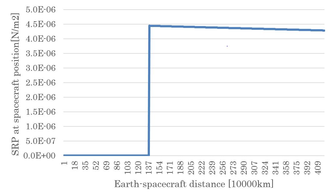
2. Verification of calculation in CalcShadowFunction function
1. overview
- The calculation of the shadow function is verified.
- The result of the
CalcShadowFunctionof S2E is compared with the results of thesolar intensityof STK.
2. conditions for the verification
-
Orbit
- The orbit of the ISS was used for verification.
- The TLE data are as follows.
1 25544U 98067A 20250.86981481 .00000008 00000-0 82464-5 0 9991 2 25544 51.6470 304.2415 0002004 86.5035 251.6018 15.49214189244677 -
Simulation time
- The simulation time is as follows.
//Simulation start date,[UTC]
StartYMDHMS=2020/09/13 12:00:00.0
//Simulation finish time,[sec]
EndTimeSec=3600
3. Results
- The calculation of the shadow function is verified.
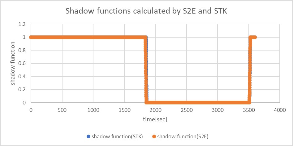
4. References
- Montenbruck, O., Gill, E., & Lutze, F. (2002). Satellite orbits: models, methods, and applications. Appl. Mech. Rev., 55(2), B27-B28.
Specification for Atmosphere model
1. Overview
1. Functions
- The
Atmosphereclass calculates an air density at the satellite's position.
- Related files
src/environment/local/atmosphere.cpp, .hppAtmosphereclass is defined.
src/environment/local/local_environment.cpp, .hppAtmosphereclass is used here as a member variable ofLocalEnvironmentclass.
src/library/external/nrlmsise00/wrapper_nrlmsise00.cpp, .hpp- An air density is calculated using an external library, NRLMSISE00 atmosphere model.
3. How to use
- Select a model and set a standard deviation as
air_density_standard_deviationfor random noise in thelocal_environment.inifile- Model
STANDARD- The air density is calculated using scale height.
HARRIS_PRIESTER- The air density is calculated using the Harris-Priester model.
NRLMSISE00- The air density is calculated using the NRLMSISE00 model.
- If users use this model, the following additional parameters must be set in the
.inifile.nrlmsise00_table_file: The space weather table pathis_manual_parameter_used: The manual setting parameter defined as follows are used or not- manual_daily_f107: User defined f10.7 (1 day)
- manual_average_f107: User defined f10.7 (30 days average)
- manual_ap: User defined ap
- Model
- The public functions
CalcAirDensity_kg_m3: Update the air density (kg/m3) based on the selected modelGetAirDensity_kg_m3: Return the calculated air density (kg/m3)
2. Installation of NRLMSISE00
- Please check How to download and compile NRLMSISE00 Library
3. Explanation of Algorithm
STANDARD
1. Air density calculation
-
Inputs
- Altitude
-
Outputs
- Air density
-
Algorithm
The STANDARD model assumes the air density as follows.
\[ \rho \left(h \right) = \rho_0 \exp \left(-\frac{h - h_0}{H} \right) \] where $h_0$ is a reference height, $\rho_0$ is an air density at the reference height, and $H$ is a scale height. These parameters are referred from the table shown in References [2].
NRLMSISE00
Read Space weather table
F10.7andKp/Apindex, which indicates the solar activity cycle, are necessary as inputs for NRLMSISE00.
These parameters, which are only during the simulation period, are read from SpaceWeather.txt.- Note
- If SpaceWeather.txt cannot be read, the atmosphere model is automatically set to STANDARD.
- SpaceWeather.txt includes data between 2015 and 2044. If the simulation date is out of range, the air density cannot be calculated accurately.
Air density calculation
- Inputs
- Decimal year
- Latitude
- Longitude
- Altitude
- Outputs
- Air density
- Algorithm
- Please refer the following reference.
- Picone, J. M.; Hedin, A. E.; Drob, D. P.; Aikin, A. C. (2002-12-01). “NRLMSISE-00 empirical model of the atmosphere: Statistical comparisons and scientific issues”. Journal of Geophysical Research: Space Physics 107 (A12)
- Please refer the following reference.
4. Verification
NRLMSISE00
-
Overview
- The calculated air density was compared with outputs from web-based NRLMSISE00 model.
-
Conditions for the verification
- input file
- Default initialize files
- initial values
- Case1 : Default initialize files
simulation_start_time_utc = 2020/01/01 11:00:00.0 simulation_duration_s = 200 simulation_step_s = 0.1 orbit_update_period_s = 0.1 log_output_period_s = 0.1 simulation_speed_setting = 0- Case2 : Start year only was changed to 2015.
simulation_start_time_utc = 2015/01/01 11:00:00.0 simulation_duration_s = 200 simulation_step_s = 0.1 orbit_update_period_s = 0.1 log_output_period_s = 0.1 simulation_speed_setting = 0- Especially, we chose following TLE for orbit calculation
tle1=1 38666U 12003B 12237.00000000 +.00000100 00000-0 67980-4 0 00008 tle2=2 38666 098.6030 315.4100 0000010 300.0000 180.0000 14.09465034 0011 -
Results
- The calculated air density at t = 0.5 [s] was compared with the result of web-based model.
- S2E
- Case1 : 2.27E-15 kg / m3
- Case2 : 1.01E-14 kg / m3
- Web-based NRLMSISE00
-
Case1 : 2.454E-15 kg / m3
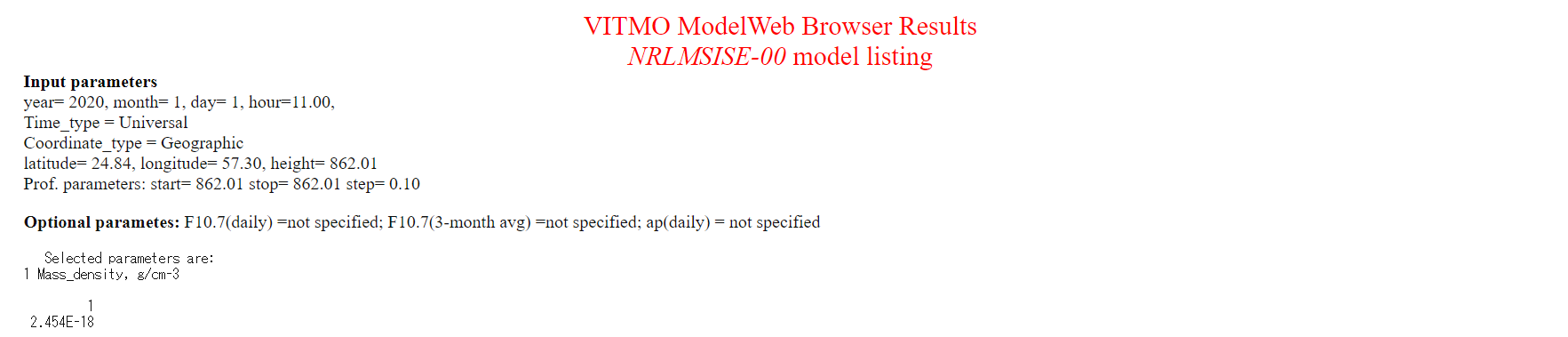
-
Case2 : 1.000E-14 kg / m3
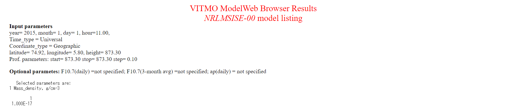
-
5. References
- Picone, J. M.; Hedin, A. E.; Drob, D. P.; Aikin, A. C. (2002-12-01). “NRLMSISE-00 empirical model of the atmosphere: Statistical comparisons and scientific issues”. Journal of Geophysical Research: Space Physics 107 (A12)
- 半揚稔雄,ミッション解析と軌道設計の基礎,現代数学社, p.324 (in japanese)
- NRLMSISE-00 Atmosphere Model , https://ccmc.gsfc.nasa.gov/modelweb/models/nrlmsise00.php
Magnetic Environment
Specification for Hipparcos catalogue
1. Overview
- This class read the csv file of Hipparcos catalogue and to enable other classes to use the data.
- Specify the max visual magnitude to read in
sample_simulation_base.ini
1. functions
ReadContents- Function to read
hip_main.csv
- Function to read
Getfunctions
- Functions to access the data of
HipparcosCataloguefrom outside of this class
2. files
HipparcosCatalogue.cpp,HipparcosCatalogue.hpp- Definitions and declarations of the class
sample_simulation_base.ini- Parameters for initialization
hip_main.csv- This is the original data of the Hipparcos catalogue. It is in the
ExtLibrariesdirectory. This data is sorted in of the visual magnitude, not in the order of HIP ID.
- This is the original data of the Hipparcos catalogue. It is in the
3. How to download hip_main.csv
s2e-core/scripts/download_HIPcatalogue.shis the script to download it. Run the following code using Git bash ins2e-core/scripts/.- NOTE for Mac OS users: Run the following script not from the Mac terminal but the Ubuntu terminal in Docker. (Because the specification of
sedis different between Mac and Linux, the file cannot be generated correctly. Reference: https://qiita.com/catfist/items/1156ae0c7875f61417ee)
bash download_HIPcatalogue.sh- NOTE for Mac OS users: Run the following script not from the Mac terminal but the Ubuntu terminal in Docker. (Because the specification of
4. How to use
- Set the parameters in
sample_simulation_base.ini - Create an instance by using initialization function
InitHipparcosCatalogue - Run
GetContentsto read the csv file - Get the data from outside this class using
Getfunctions. - The
HipparcosDatastructure has four elements, hipparcos_id, visible_magnitude, right_ascension_deg, declination_deg.HipparcosCataloguestores the data as a vector ofHipparcosData.
2. Explanation of Algorithm
TBW
3. Result of verification
The verification using this class is conducted in Spec_Telescope.md.
Specification for GNSS
1. Overview
1. function
- A class to read data about orbit and clock bias of GNSS satellites such as .sp3 and .clk_30s and use them in other classes.
- Determine the file name of GNSS satellites' data and time from
[GNSS_SATELLITES]insample_gnss.ini.
2. Related files
src/environment/global/globalEnvironment.cpp, .hpp- GnssSatellites class is defined. Various GET functions are also implemented.
src/environment/global/initialize_gnss_satellites.cpp, .hpp- This makes the instance of the GnssSatellites class. The initialization is described in the
sample_gnss.inifile.
- This makes the instance of the GnssSatellites class. The initialization is described in the
ExtLibraries/sp3- It contains a set of files (.sp3, .clk_30s) necessary for generating orbits and clock biases.
3. About downloading .sp3 files, etc.
- The author has not yet written script files to download .sp3 or .clk. Users can download them from
ftp://igs.ensg.ign.fr/pub/igs/products/,http://mgmds01.tksc.jaxa.jp/, etc., referring to the directory classification. The directories are assumed to be as follows.
ExtLibraries
    |
   sp3
    ├── CODE
    │   └── final
    ├── IGS
    │   ├── igl
    │   ├── igr
    │   │   └── clk
    │   ├── igs
    │   │   └── clk_30s
    │   └── igu
    ├── JAXA
    │   ├── final
    │   ├── madoca
    │   ├── rapid
    │   └── ultra_rapid
    └── QZSS
        ├── final
        ├── rapid
        └── ultra_rapid
2. How to use
-
Parameters, which file to use or else are set in
sample_gnss.inidirectory_path: fixedcalculation: whether to use this GNSS classtrue_position_file_sort: Select the type of file to generate the true value of the GNSS satellite coordinates.true_position_first: The first file to readtrue_position_last: The last file to readtrue_position_interpolation_method: Select the interpolation methodtrue_position_interpolation_number: Select the number of points to be interpolated, so the order of the function will betrue_position_interpolation_number-1.true_clock_file_extension: Whether to use .sp3 or clock-only files such as .clk_30s
estimationparameters are the same as above. -
Users can retrieve the coordinates and clock bias of each GNSS satellite with the provided
Getfunctions.
3. Algorithm
Basically, the trajectory is generated by interpolation, but some data are often missing, so we have dealt with it. For the coordinates, the trajectory is generated by interpolation from the available coordinates, and for the clock bias is generated by extracting only the strictly surrounding values.
- Extract the contents of the file with
initialize_gnss_satellites.cpp. - Create a table for generating coordinates and clock bias with
Init().time_table_: The Unix Time of all times are listed.gnss_*_table_*: Contains the coordinates or clock bias values at all times.available_table_: Whether available of the data of all satellites at all timestime_and_index_list_: Contains the pair of available time and the index in the table.
SetUp(): Set the first interpolation reference location fromtime_table_andtime_and_index_list_, set the index of the reference tonearest_index_(used later in Update).time_vector_,ecef_,eci_,clock_arestd::vectorused for interpolation calculation.Update(): Coordinates and clock bias are calculated based on the time. Thetime_vector_,ecef_,eci_, andclock_, which are used as the basis of interpolation, are updated according to the nearest time.
4. Result and Specification
Some of the calculated ECI coordinates are shown below.
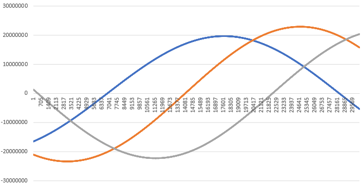
Specification of Earth Rotation
1. Overview
1. Functions
- The
EarthRotationclass calculates the rotational motion of the Earth.
2. Related files
src/environment/global/earth_rotation.cpp, .hppEarthRotationclass is defined here.
src/environment/global/celestial_information.cpp, .hppEarthRotationclass is used here.
3. How to use
- Make an instance of the
EarthRotationclass inCelestialInformationclass. - Select rotation mode in
sample_simulation_base.iniIDLE: no motion ( $\mathrm{DCM_{ECItoECEF}}$ is set as the unit matrix)- If the rotation mode input is neither
FULLnorSIMPLE, theIDLEmode is set.
- If the rotation mode input is neither
SIMPLE: axial rotation only ( $\mathrm{DCM_{ECItoECEF}} = \bf{R}$ )FULL: Precession and Nutation are taken into account ( $\mathrm{DCM_{ECItoECEF}} = \bf{R}\bf{N}\bf{P}$ )- $\bf{R}$, $\bf{N}$, $\bf{P}$ stand for the DCM of axial rotation, nutation, precession, respectively.
2. Explanation of Algorithm
The algorithm is based on IERS Conventions 2003.
1. Update
1. overview
- This function calculates the coordinate transformation from ECI to ECEF, calling
RotationandPrecessionandNutationfunctions. \[ \mathrm{DCM_{ECItoECEF}} = \bf{R}\bf{N}\bf{P} \] - where $\bf{R}$, $\bf{N}$, $\bf{P}$ stand for the DCM of axial rotation, nutation, precession, respectively.
2. inputs and outputs
- Input
- Julian date
- Output
- the DCM of the coordinate transformation from ECI to ECEF
3. algorithm
\[ \mathrm{jdTT} = \mathrm{julian, date} + \mathrm{dtUT1UTC} \]
- where Julian date is the input, dtUT1UTC is the time difference between UT1 and UTC
- dtUT1UTC = 32.184 [s]
\[ \mathrm{tTT} = \frac{\mathrm{jdTT} - \mathrm{JDJ2000}}{\mathrm{JC}} \]
-
where tTT is Julian century for terrestrial time, JDJ2000 is Julian Date @ J2000, JC is Julian Century
- JDJ2000 = 2451545.0 [day]
- JC = 36525 [day/century]
-
By using tTT, we get the DCM of precession ( $\bf{P}$ ) and nutation ( $\bf{N}$ ) with
PrecessionandNutationfunctions. -
$\varepsilon$, $\Delta \varepsilon$, $\Delta \psi$ are calculated in
Nutationfunction.
\[ \begin{align} \mathrm{E_q} &= \Delta \psi \cos{(\varepsilon + \Delta \varepsilon)} \\ \mathrm{GAST} &= \mathrm{GMST} + \mathrm{E_q} \end{align} \]
-
where GAST is Greenwich Apparent Sidereal Time, GMST is Greenwich Mean Sidereal Time
-
GAST is calculated from julian date in
gstimefunction insrc/Library/sgp4/sgp4unit.h. -
By using GMST, We get the DCM of axial rotation ( $\bf{R}$ ) with the
Rotationfunction. The coordinate transformation from ECI to ECEF is calculated. \[ \mathrm{DCM_{ECItoECEF}} = \bf{R}\bf{N}\bf{P} \]
4. note
- If rotation mode is
Simple, only axial rotation is calculated.
2. AxialRotation
1. overview
- This function calculates the axial rotation of the central object.
2. inputs and outputs
- Input
- Greenwich Apparent Sidereal Time (GAST)
- Output
- the DCM of axial rotation ( $\bf{R}$ )
3. algorithm
\[ \bf{R} = \begin{pmatrix} \cos{\mathrm{(GAST)}} & \sin{\mathrm{(GAST)}} & 0 \\
- \sin{\mathrm{(GAST)}} & \cos{\mathrm{(GAST)}} & 0 \\ 0 & 0 & 1 \end{pmatrix} \]
3. Precession
1. overview
- This function calculates the precession of the central object.
2. inputs and outputs
- Input
- Julian century for terrestrial time (tTT)
- Output
- the DCM of precession ( $\bf{P}$ )
3. algorithm
- Precession angles are calculated as follows.
\[ \begin{align} \zeta &= 2306.2181" \mathrm{tTT} + 0.30188" \mathrm{tTT}^2 + 0.017998" \mathrm{tTT}^3 \\ \theta &= 2004.3109" \mathrm{tTT} - 0.42665" \mathrm{tTT}^2 - 0.041833" \mathrm{tTT}^3 \\ z &= 2306.2181" \mathrm{tTT} + 1.09468" \mathrm{tTT}^2 + 0.018203" \mathrm{tTT}^3 \\ \end{align} \] \[ \bf{P} = \begin{pmatrix} \cos{(-z)} & \sin{(-z)} & 0 \\- \sin{(-z)} & \cos{(-z)} & 0 \\ 0 & 0 & 1 \end{pmatrix} \begin{pmatrix} \cos{\theta} & 0 & - \sin{\theta} \\ 0 & 1 & 0 \\ \sin{\theta} & 0 & \cos{\theta} \end{pmatrix} \begin{pmatrix} \cos{(-\zeta)} & \sin{(-\zeta)} & 0 \\
- \sin{(-\zeta)} & \cos{(-\zeta)} & 0 \\ 0 & 0 & 1 \end{pmatrix} \]
4. Nutation
1. overview
- This function calculates the nutation of the central object.
2. inputs and outputs
- Input
- Julian century for terrestrial time (tTT)
- Output
- Return: the DCM of precession ( $\bf{N}$ )
- $\varepsilon$: mean obliquity of the ecliptic
- $\Delta \varepsilon$: nutation in obliquity
- $\Delta \psi$: nutation in longitude
3. algorithm
Delaunay angles are calculated as follows. \[ \begin{align} l &= 134.96340251^\circ + 1717915923.2178"\mathrm{tTT} + 31.8792"\mathrm{tTT}^2 + 0.051635"\mathrm{tTT}^3 - 0.00024470"\mathrm{tTT}^4 \\ l' &= 357.52910918^\circ + 129596581.0481"\mathrm{tTT} - 0.5532"\mathrm{tTT}^2 + 0.000136"\mathrm{tTT}^3 - 0.00001149"\mathrm{tTT}^4 \\ F &= 93.27209062^\circ + 1739527262.8478"\mathrm{tTT} - 12.7512"\mathrm{tTT}^2 - 0.001037"\mathrm{tTT}^3 + 0.00000417"\mathrm{tTT}^4 \\ D &= 297.85019547^\circ + 1602961601.2090"\mathrm{tTT} - 6.3706"\mathrm{tTT}^2+0.006593"\mathrm{tTT}^3 -0.00003169"\mathrm{tTT}^4 \\ \Omega &= 125.04455501^\circ - 6962890.5431"\mathrm{tTT} + 7.4722"\mathrm{tTT}^2+0.007702"\mathrm{tTT}^3-0.00005939"\mathrm{tTT}^4 \\ \end{align} \]
- l : mean anomaly of the moon
- l' : mean anomaly of the sun
- F : mean argument of latitude of the moon
- D : mean elongation of the moon from the sun
- $\Omega$ : mean longitude of ascending node of the moon
$\varepsilon$ and $\Delta \varepsilon$ and $\Delta \psi$ are calculated as follows.
\[ \begin{align} \varepsilon &= 23^\circ26'21".448 - 46".8150\mathrm{tTT} - 0".00059\mathrm{tTT}^2 + 0".001813\mathrm{tTT}^3 \\ \Delta \epsilon &= 9.205\cos{\Omega} + 0.573\cos{2L'} - 0.090\cos{2\Omega} + 0.098\cos{2L}+0.007\cos{l'} - 0.001\cos{l} + 0.022\cos{(2L'+l')} + 0.013\cos{(2L+l)}-0.010\cos({2L'-l')} , [\mathrm{arcsec}] \\ \Delta \psi &= -17.206\sin{\Omega} - 1.317\sin{2L'} + 0.207\sin{2\Omega} - 0.228\sin{2L} + 0.148\sin{l'}+0.071\sin{l}-0.052\sin{(2L'+l')} - 0.030\sin{(2L+l)}+0.022\sin{(2L'-l')} , [\mathrm{arcsec}] \\ \end{align} \]
where $L = F + \Omega$,$L' = L - D$
\[ \bf{N} = \begin{pmatrix} 1 & 0 & 0 \\ 0 & \cos{\left(-(\varepsilon + \Delta \varepsilon)\right)} & \sin{\left(-(\varepsilon + \Delta \varepsilon)\right)} \\ 0 & - \sin{\left(-(\varepsilon + \Delta \varepsilon)\right)} & \cos{\left(-(\varepsilon + \Delta \varepsilon)\right)} \end{pmatrix} \begin{pmatrix} \cos{(-\Delta \psi)} & \sin{(-\Delta \psi)} & 0 \\
- \sin{(-\Delta \psi)} & \cos{(-\Delta \psi)} & 0 \\ 0 & 0 & 1 \end{pmatrix} \begin{pmatrix} 1 & 0 & 0 \\ 0 & \cos{\varepsilon} & \sin{\varepsilon} \ 0 & - \sin{\varepsilon} & \cos{\varepsilon} \end{pmatrix} \]
3. Results of verifications
1. $\mathrm{DCM_{ECItoECEF}}$ calculation in Update function
1. overview
- The $\mathrm{DCM_{ECItoECEF}}$ calculation is compared with Matlab's dcmeci2ecef function
2. conditions for the verification
- input value
- Simulation time
- 200, 20000, 100000 [s]
- other conditions
- default initialize files
- UTC = 2020/01/01 12:00:00
- Step Time 0.1 [s]
- default initialize files
- Simulation time
3. results
-
Results of calculation time in S2E
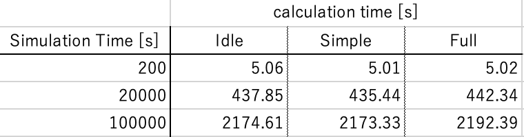
If you want to reduce the calculation time, it is recommended to select Simple mode rather than Idle mode. Note again that if the rotation mode input is neither Full nor Simple, the Idle mode is set.
-
Results of S2E in
Simplerotation mode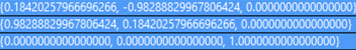
-
Results of S2E in
Fullrotation mode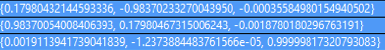
-
Results of Matlab
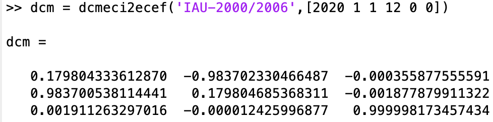
The results of Full rotation mode and Matlab agree well. Note that Matlab is based on the IAU-2000/2005 reference system, while S2E is based on IERS Conventions 2003.
4. References
- 天体の回転運動理論入門講義ノート, 福島 登志夫, 2007.(written in Japanese)
- 天体の位置計算, 長沢 工, 2001.(written in Japanese)
- IERS Conventions 2003, D. D. McCarthy and G Petit, 2003.
- MATLAB dcmeci2ecef, retrieved June 18, 2021.
Specification of Power Port
1. Overview
1. Functions
PowerPortclass provides features of an electrical power connection.- Users can use the class to control the electrical power switching of components and calculate the component's consumed electrical current.
2. Related files
- Main files:
power_port.cpp, .hpp - Referenced files:
component.cpp, .hppandpower_control_unit.cpp, .hpp
3. How to use
- Example: The
sample_components.hppin thes2e-core/simulation_sample/spacecraft/is helpful to know how to use the feature. - Make a component class that inherits the
Componentclass.- The
Componentclass has thePowerPortclass as a member and controls the component's action according to the electrical power switches.
- The
- Make an instance of
PowerControlUnitand connect the power port.- The
PowerControlUnitbase class has a member of themapof thePowerPortclass and manages the port id and connection of thePowerPort. - Users can make their PCU by inheriting the
PowerControlUnitbase class and can control the power switching in theMainRoutinefunction.
pcu_ = new PowerControlUnit(clock_gen); pcu_->ConnectPort(0, 0.5, 3.3, 0.3); - The
- Make an instance of the components with the connected
PowerPort.obc_ = new OnBoardComputer(1, clock_gen, pcu_->GetPowerPort(0)); - Control the power switches by using the
PowerControlUnit.- The default setting of the power switch is
off, so users need to power on the port to execute theMainRoutineof the components.
pcu_->GetPowerPort(0)->SetVoltage(3.3); - The default setting of the power switch is
- Note: The virtual power port is created when users make an instance of the
Componentclass and its subclasses without thePowerPortinformation. The virtual port has a minus value port ID, and the switch state is originallyON, but the consumed power is zero.
2. Explanation of Algorithm
1. SetVoltage
1. overview
- This function is a setter function of the supply voltage to the power port.
- Users can control the power switch by using this function.
2. inputs and outputs
- input: supply voltage to the port
- output: switch state of the port
3. algorithm
- After the voltage is set, the
Updatefunction is called to check that the supply voltage is enough to turn on the component.
4. note: N/A
1. Update
1. overview
- This is an update function of the switch state and the consumed current.
- This function also has an over-current protection feature.
2. inputs and outputs
- input: N/A (members of the class)
- output: switch state of the port
3. algorithm
- When the supply voltage is larger than the
kMinimumVoltageof the component, the switch state becomestrue, and the consumed current is calculated as the following equation. \[ I = P/V \] - The
Pis theassumed_power_consumption, and users can set the value with theSetAssumedPowerConsumptionfunction. - If the calculated current consumption is larger than the
kCurrentLimit, the over-current protection feature is executed and turning the switch off.
4. note: N/A
3. Results of verifications
N/A
4. References
N/A
Monte Carlo Simulation
1. Overview
1. Functions
- The
Monte Carlo Simulationfeature of S2E provides a framework for Monte Carlo simulation
2. Related files(TBW)
src/simulation/monte_carlo_simulationinitialize_monte_carlo_parameters: A class to initialize randomized parametersinitialize_monte_carlo_simulationmonte_carlo_simulation_executor: The main class for Monte Carlo simulationsimulation_object:
data/sample/initialize_files/sample_simulation_base.ini
3. How to use
2. Explanation of Algorithm
TBW
3. Results of verifications
TBW