Specification for Orbit dynamics with RK4 propagation
1. Overview
1. functions
- The
Rk4OrbitPropagationclass calculates the position and velocity of satellites with 4th Order Runge-Kutta method(RK4).
2. files
src/dynamics/orbit/orbit.hpp, cpp- Definition of
Orbitbase class
- Definition of
src/dynamics/orbit/initialize_orbit.hpp, .cpp- Make an instance of orbit class.
src/dynamics/orbit/rk4_orbit_propagation.hpp, .cpp
3. How to use
- Select
propagate_mode = RK4in the spacecraft's ini file. - Select
initialize_modeas you want.DEFAULT: Use default initialize method (RK4andENCKEuse position and velocity,KEPLERuses init_mode_kepler)POSITION_VELOCITY_I: Initialize with position and velocity in the inertial frameORBITAL_ELEMENTS: Initialize with orbital elements
2. Explanation of Algorithm
1. Propagate function
- The position and velocity of the satellite are updated by using RK4. As the input of RK4, the six-state variables are set. These state variables are the three-dimensional position [$x$, $y$ ,$z$] and three-dimensional velocity [$v_x$, $v_y$, $v_z$] at the inertial coordinate. Here, the inertial coordinate is decided by the
PlanetSelect.ini - As the force which works to the satellite motion is the external acceleration [$a_x$,$a_y$,$a_z$] calculated from the disturbance class or thruster class and the gravity force from the center planet, which is defined in
PlanetSelect.ini. As a summary, the orbit is calculated as the following equation. \[ \begin{align} \dot{x} &= v_x\\ \dot{y} &= v_y\\ \dot{z} &= v_z\\ \dot{v}_x &= a_x-\mu\frac{x}{r^3}\\ \dot{v}_y &= a_y-\mu\frac{y}{r^3}\\ \dot{v}_z &= a_z-\mu\frac{z}{r^3}\\ r &= \sqrt{x^2+y^2+z^2} \end{align} \]
3. Results of verifications
1. Verification of the error of Fourth Order Runge-Kutta method (RK4)
1. Overview
- Verify the numerical integration error of the RK4 method.
- The output of the simulation was compared with the analytical solution.
2. conditions for the verification
- The Verifications were conducted in the case of
simulation_step_sandorbit_update_period_swere 0.1(sec), 1(sec), and 10(sec). - The initial values of the propagation are as follows:
initial_position_i_m(0) = 1.5944017672e7 initial_position_i_m(1) = 0.0 initial_position_i_m(2) = 0.0 initial_velocity_i_m_s(0) = 0.0 initial_velocity_i_m_s(1) = 5000.0 initial_velocity_i_m_s(2) = 0.0 - This is a circular orbit, which period is about 20040(sec). The center of the orbit is Earth.
- As a reference, the analytical solution was used. The solution is as follows: \[ x=R\cos(\omega t),y=R\sin(\omega t)\quad when~R=1.5944017672\times10^7, \omega=0.000313597243985794 \]
- All of the effects of disturbance and environment were disabled.
- The simulation time is 60120(sec), which is approximately three-period. In addition, for a long-term test, the case in which simulation time is 200400(about 10 periods) was tested. The
orbit_update_period_sof this case is 1(sec).
3. results
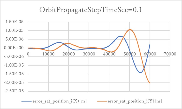
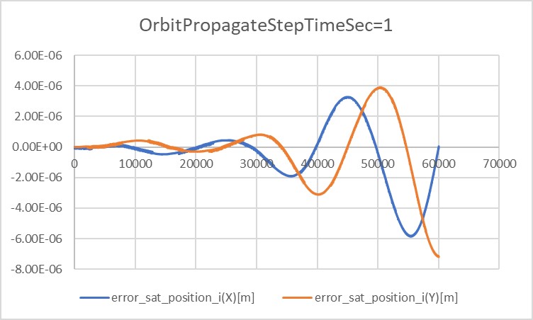
- In the cases of
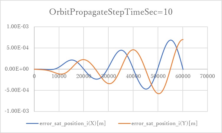
orbit_update_period_s=0.1andorbit_update_period_s=1, the error is kept within $10^{-6}$ order. However, once the error grows, it will get bigger and bigger. - In the case of
orbit_update_period_s=10, the error quickly grows up to $10^{-4}$ order.
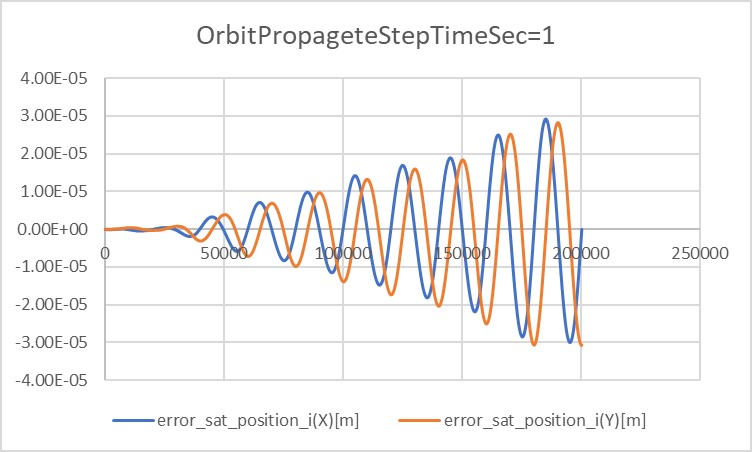
- In the long-term test result, it is clear that the error magnitude grows proportionally to the time.
4. Others
- At first, the output of STK would be used for reference. However, it did not work well. Data were input as follows:
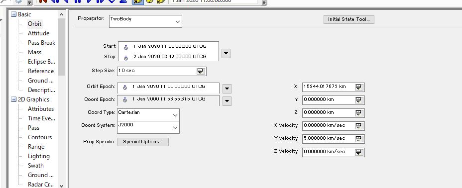
- However, the result is as follows:
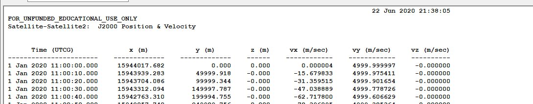
- As this figure shows, the initial values in the result are slightly different from the input.
- In the .sa files, the initial values of $x, y, z, v_x, v_y, v_z$ are converted into elements of orbit and stored. The error might occur in the process of this conversion.
4. References
NA